1. Introduction to biological circuit design
Key concepts
Genetic circuits are sets of interacting molecules that control cellular behaviors
Circuit design principles provide functional rationales for choosing one circuit design or architecture over another, and are usually of the form Feature X provides function Y.
Executable Jupyter notebooks (like this one) enable exploration of key concepts throughout this course.
Ordinary differential equations for protein production and removal allow analysis of simple gene expression processes.
Separation of time scales simplifies analysis of many circuits.
Gene regulation circuits can be analyzed in terms of binding of activators and repressors to binding sites.
[1]:
# Colab setup ------------------
import os, sys, subprocess
if "google.colab" in sys.modules:
    cmd = "pip install --upgrade watermark"
    process = subprocess.Popen(cmd.split(), stdout=subprocess.PIPE, stderr=subprocess.PIPE)
    stdout, stderr = process.communicate()
# ------------------------------

import numpy as np
import bokeh.io
import bokeh.plotting

bokeh.io.output_notebook()
Biological circuit design
The living cell is an incredible device: It can sense its environment, search out nutrients, avoid threats, control its own division and growth, and keep track of time. Cells can coordinate with other cells to build multicellular tissues and organs, including brains, develop into multifunctional organisms, and generate immune systems that can patrol those organisms to repair damage and destroy pathogens. For the most part, they do these things reliably and without complaining. All of these behaviors are largely implemented by circuits of interacting proteins, DNA, RNA, and other molecules.
In this course, we will study these biological circuits from a design point of view – we will try to understand a wide range of different circuit architectures and how they provide specific functions for the cell.
Beyond molecular biology:
Historically, the framework of molecular biology became dominant in the 1950s, with the central idea that we could understand biological phenomena in terms of the molecular structure and biochemical function of DNA, mRNA, and other molecules. (Read “The Eighth Day of Creation” for an excellent history of molecular biology.) But it was quickly recognized that these molecules formed circuits. For example, in a 1962 essay, speaking about the organization of transcriptional regulatory systems, Jacob and Monod wrote,
It is obvious from the analysis of these [bacterial genetic regulatory] mechanisms that their known elements could be connected into a wide variety of ‘circuits’ endowed with any desired degree of stability. Jacob F, Monod J, “On the regulation of gene activity,” Symposium on cellular regulatory mechanisms, 1962.
Around the 2000s, interest in the structure and function of circuits began to explode, fueled in part by new technologies that improved the ability to make quantitative, high-throughput measurements of biological systems. The new field took the name systems biology.
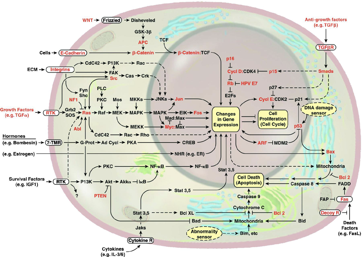
This image of the cell as a set of circuits comes from a classic review of cancer by Hanahan and Weinberg, Cell, 2000.
What is a biological circuit?
For this course, we will think about at least two levels of biological circuitry:
Molecular circuits consist of molecular species (genes, proteins, etc.) that interact with one another in specific ways. For example, a given gene can be transcribed to produce a corresponding mRNA, which can in turn be translated to produce a specific protein. That protein may be a repressor that turns off expression of a different gene, or even its own gene. Similarly, a kinase may phosphorylate a specific target protein, altering its ability to catalyze a reaction or modify another protein. The molecular specificity of these interactions – analogous to wires in electronics – is the key property that enables them to form molecular circuits.
One level up, we will also consider cell circuits. In this case, cells in different states, of different types, or even from different species signal to one another to control each other’s growth, death, proliferation, and differentiation. The key variables in these circuits are the population sizes and spatial arrangements of each type of cell. For example, the immune system, in which different cell types influence each other’s proliferation and differentiation through cytokines and other signals, represents a collection of complex, interconnected cell circuits.
The two levels are not independent. The behavior of each cell type within a cell circuit is determined by the structure of its molecular circuits.
At either level, we can also distinguish between natural circuits and synthetic circuits. The former are discovered in microbes, plants, and animals, while the latter are designed and engineered in cells out of well-characterized, re-engineered, or de novo designed genes, proteins, and other molecular components.
Biological circuit design
Design problems emerge whenever one can build many different products from arrangements of the same elements. Electronic circuits are composed of a handful of different kinds of elements: transistors, resisters, capacitors, etc. that can be connected in different ways to produce circuits with different properties. Design requires comparing different circuit designs that may appear to perform similar functions, but in fact exhibit different tradeoffs, e.g. between power and performance, or speed and precision. Design problems are also prevalent outside of science and engineering. For example, to make a movie poster one has to choose and arrange graphical elements in relation to one another.
We now have much information about the molecular components of cells (genes, RNAs, proteins, metabolites, and many other molecules) and their interactions. In many cases, we know the sites at which transcription factors bind genome-wide, which proteins chemically modify which others, and which proteins function together in complexes. It might seem as if we ought to already be able to understand, predict, and control cellular circuits with great precision. However, fundamental questions about the designs of these circuits still remain unclear. For example:
What capabilities does each circuit provide for the cell? (function, design principles)
How do these capabilities emerge from circuit architecture? (mechanism)
How can we control cells in predictable ways using these circuits? (biomedical applications)
How can we use circuit design principles to program predictable new behaviors in living cells? (synthetic biology and bioengineering)
In this course, we will address these questions for both natural and synthetic circuits, with the idea that the principles that allow a circuit to function effectively within or among cells do not necessarily depend on whether that circuit evolved naturally or is constructed in the lab. Having said that, we also recognize that evolution may be able to produce designs that are more complex or different from those we are currently able to construct, or even conceive. In fact, a major goal of the course is to see to what extent we can learn principles from natural circuits that will allow us to design synthetic circuits more effectively.
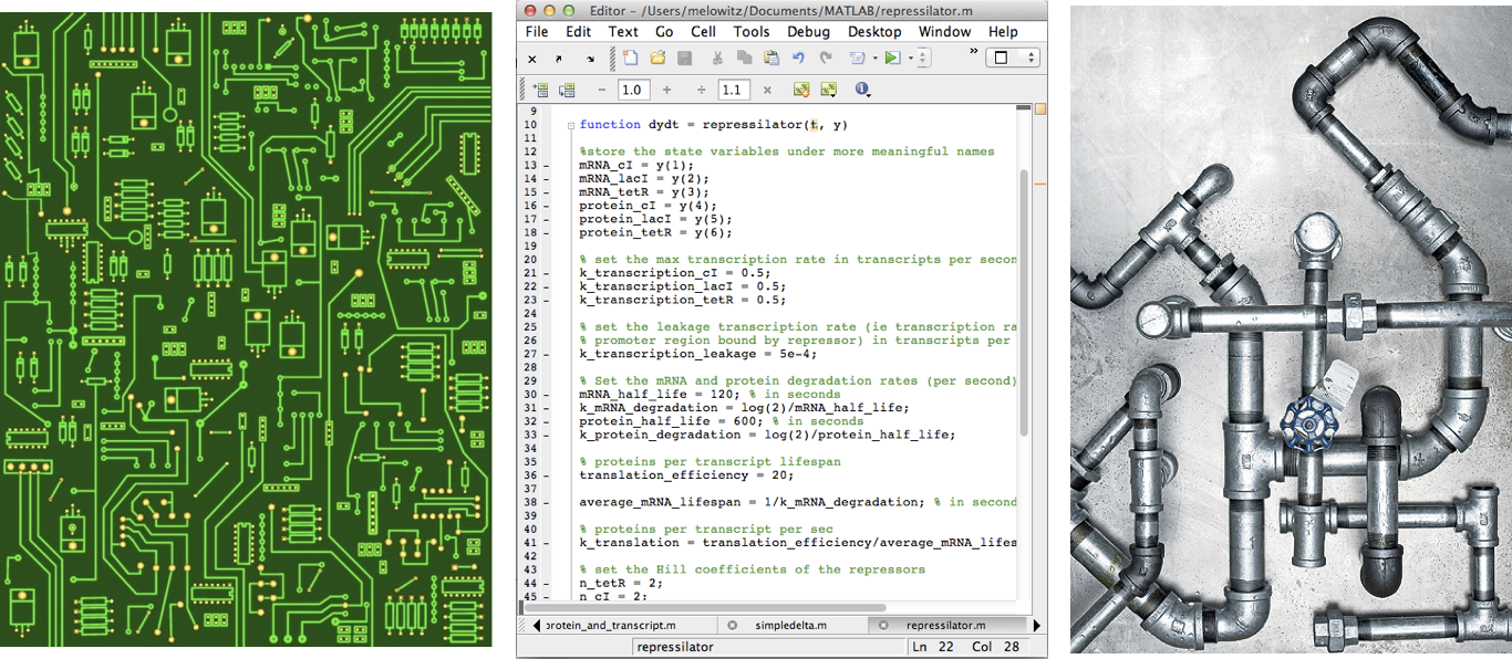
Electronics, software, and plumbing are great examples of human-designed systems that possess many properties analogous to biological circuits. These systems are based on known design principles that sometimes overlap with, and sometimes differ from, those of biological circuits.
Biological circuits differ from many other types of circuits or circuit-like systems
Is biological circuit design a solved problem? Electronics, software, plumbing, construction, and other human designed systems are based on connections between modular components (see Figure). Can we not just apply known principles of those systems biological circuits? The answer is generally “no,” or “only a little,” because biological systems differ in fundamental ways from these systems:
Natural circuits were not designed by people. They evolved. That means they are not “well-documented” and their function(s) are often totally unclear.
Even synthetic circuits, which are designed by people, often use evolved components (such as transcription factors) that do not fully understand.
Biological circuits use fundamentally different designs than human-engineered counterparts. For example, in cells, molecular components exhibit extensive many-to-many interactions (“crosstalk”) among their components. This property is typically avoided in electronics but may provide unique capabilities to cells.
Noise: While electronic circuits can function deterministically, biological circuits function with high levels of stochastic (random) fluctuations in their own components. These fluctuations are often called “noise.” And noise is not just a nuisance: some biological circuits take advantage of it to enable behaviors that would not be possible without it.
Biological circuits use parallelism: The same circuit can operate in many different genetically identical individual cells, whether in a bacterial population or in a multicellular organism.
Electrical systems use positive or negative voltages and currents, allowing for positive or negative effects. By contrast, biological circuits are built out of molecules (or cells) whose concentrations cannot be negative. That means they must use other mechanisms for “inverting” activities.
From a more practical point of view, we have a very limited ability to construct, test, and compare designs. Even with recent developments such as CRISPR, our ability to rapidly and precisely produce cells with well-defined genomes remains limited compared to what is possible in more advanced disciplines. (This situation is rapidly improving!)
What other fundamental differences between biological circuits and human designed systems can you think of?
Inspiration from electronics
In their classic book, The Art of Electronics, Horowitz and Hill explain something similar to the excitement many now feel now about biological circuit design:
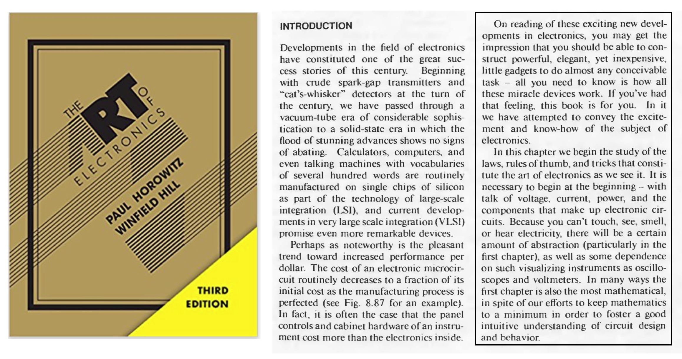
Paul Horowitz and Winfield Hill, The Art of Electronics, 3rd edition, Cambridge University Press, 2015.
Premise and goals
This course explores foundational concepts needed to understand, predict, and control living systems with greater precision (systems biology), and to design synthetic circuits that provide new functions (synthetic biology). We will develop quantitative approaches for analyzing different circuit designs (tools), and also identify circuit design principles that provide insight and intuition into how different designs operate, and why they were selected by evolution or synthetic biologists.
Design principles relate circuit features to circuit functions
We will define a circuit design principle as a statement of the form: Circuit feature X enables function Y. Each module of the course will explore a different design principle. Here are some examples:
Negative autoregulation of a transcription factor accelerates its response to a change in input.
Kinases that also act as phosphatases (bifunctional kinases) provide tunable linear amplifiers in two-component signaling systems.
Pulsing a transcription factor on and off at different frequencies (time-based regulation) can enable coordinated regulation of many target genes.
Noise-excitable circuits enable cells to control the probability of transiently differentiating into an alternate state.
Mutual inactivation of receptors and ligands in the same cell enable equivalent cells to signal unidirectionally.
Independent tuning of gene expression burst size and frequency enables cells to control cell-cell heterogeneity in gene expression.
Feedback on morphogen mobility allows tissue patterns to scale with the size of a tissue
Developing intuition: analzying the simplest gene regulation circuits
We will start with the simplest possible “circuit” – hardly a circuit at all, really – just a single gene, coding for a single corresponding protein. This minimal example will allow us to develop intuition for the dynamics of the simplest gene regulations systems and lay out a procedure that we can further extend to analyze more complex circuits.
How much protein will the gene x produce? We assume that the gene will be transcribed to mRNA and those mRNA molecules will in turn be translated to produce proteins, such that new proteins are produced at a total rate \(\beta\) molecules per unit time. The \(x\) protein does not simply accumulate over time. It is also removed both through active degradation as well as dilution as cells grow and divide. For simplicity, we will assume that both processes tend to reduce protein concentrations through a simple first-order process, with a rate constant \(\gamma\).
The approach we are taking can be described as “phenomenological modeling.” We do not explicitly represent every underlying molecular step. Instead, we assume those steps give rise to “coarse grained” relationships that we can model in a manner that is independent of many underlying molecular details. The test of this approach is whether it allows us to understand and experimentally predict the behavior of real biological systems. See Wikipedia’s article on phenomenological models and this article by Jeremy Gunawardena.
Thus, we can draw a diagram of our simple gene, x, with its protein being produced and removed (dashed circle):
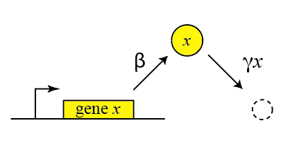
Here, protein production occurs at rate \(\beta\) and degradation+dilution at rate \(\gamma x\). We can then write down a simple ordinary differential equation describing these dynamics:
\begin{align} &\frac{dx}{dt} = \mathrm{production - (degradation+dilution)} \\[1em] &\frac{dx}{dt} = \beta - \gamma x \end{align}
where
\begin{align} \gamma = \gamma_\mathrm{dilution} + \gamma_\mathrm{degradation} \end{align}
A note on effective degradation rates: When cells are growing, protein is removed through both degradation and dilution. For stable proteins, dilution dominates. For very unstable proteins, whose half-life is much smaller than the cell cycle period, dilution may be negligible. In bacteria, mRNA half-lives (1-10 min, typically) are much shorter than protein half-lives. In eukaryotic cells this is not necessarily true (mRNA half-lives can be many hours in mammalian cells).
Solving for the steady state
Often, one of the first things we would like to know is the concentration of protein under steady state conditions. To obtain this, we set the time derivative to 0, and solve:
\begin{align} &\frac{dx}{dt} = \beta - \gamma x = 0 \\[1em] &\Rightarrow x_{\mathrm{st}} = \beta / \gamma \end{align}
In other words, the steady-state protein concentration depends on the ratio of production rate to degradation rate.
Including transcription and translation as separate steps
This description does not distinguish between transcription and translation. However, considering both processes separately can be important in the more dynamic and stochastic contexts that we will encounter later in the course. To do so, we can simply add an additional variable to represent the mRNA concentration, which is now transcribed, translated to protein, and degraded (and diluted), as shown schematically here:
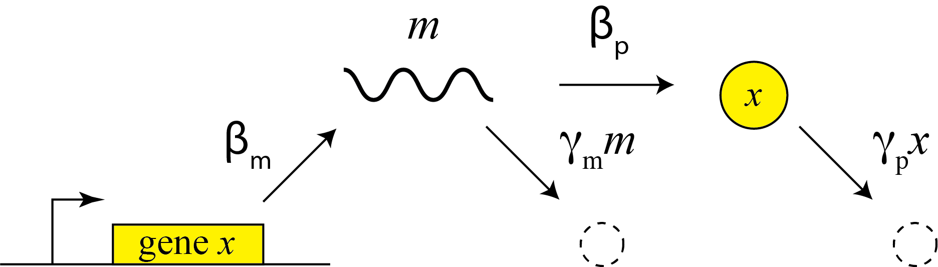
These reactions can be described by two coupled differential equations for the mRNA (m) and protein (x):
\begin{align} &\frac{dm}{dt} = \beta_m - \gamma_m m, \\[1em] &\frac{dx}{dt} = \beta_p m - \gamma_p x. \end{align}
Now, we can determine the steady state mRNA and protein concentrations straightforwardly, by setting both time derivatives to 0 and solving. We find:
\begin{align} &m_\mathrm{st} = \beta_m / \gamma_m, \\[1em] &x_\mathrm{st} = \frac{\beta_p m_\mathrm{st}}{\gamma_p} = \frac{\beta_p \beta_m}{\gamma_p \gamma_m}. \end{align}
From this, we see that the steady state protein concentration is proportional to the product of the two synthesis rates and inversely proportional to the product of the two degradation rates.
And this gives us our first design puzzle: the cell could control protein expression level in at least four different ways: It could modulate (1) transcription, (2) translation, (3) mRNA degradation or (4) protein degradation rates (or combinations thereof). Are there tradeoffs between these different options? Are they all used indiscriminately or is one favored in natural contexts?
From gene expression to gene regulation - adding a repressor
In principle, genes could be left “on” all the time. In actuality, the cell activity regulates them, turning their expression levels lower or higher depending on environmental conditions and cellular state. Repressors provide a key mechanism for regulation. Repressors are proteins that bind to cognate specific sequences at or near a promoter, to change its expression. Often the strength of repressor binding depends on external inputs. For example, the LacI repressor normally turns off the genes for lactose utilization in E. coli. However, in the presence of lactose in the media, a modified form of lactose binds to LacI, inhibiting its ability to repress its target genes. Thus, a nutrient (lactose) can regulate expression of genes that allow the cell to use it. (The book “The lac operon” by B. Müller-Hill provides the fascinating scientific and historical saga of this iconic system.)
In the following diagram, we label the repressor R.
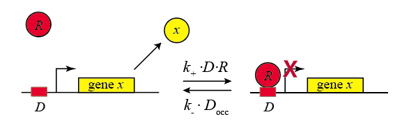
\begin{align} D + R \rightleftharpoons D_{occ} \end{align}
Within the cell, the repressor binds and unbinds its target site. We assume that the expression level of the gene is lower when the repressor is bound and higher when it is unbound. The mean expression level of the gene is then proportional to the fraction of time that the repressor is unbound.
We therefore compute the “concentration” of DNA sites in occupied or unoccupied states. (Within a single cell an individual site on the DNA is either bound or unbound, but averaged over a population of cells, we can talk about the mean occupancy of the site). Let \(D\) be the concentration of unoccupied promoter, \(D_\mathrm{occ}\) be the concentration of occupied promoter, and \(D_\mathrm{tot}\) be the total concentration of promoter, with \(D_\mathrm{tot} = D + D_\mathrm{occ}\), as required by conservation of mass.
We can also assume a separation of timescales between the rates of binding and unbinding of the repressor to the DNA binding site are both often fast compared to the timescales over which mRNA and protein concentrations vary. (Careful, however, in some contexts, such as mammalian cells, this is not true.)
All we need to know is the mean concentration of unoccupied binding sites, \(D/D_\mathrm{tot}\).
\begin{align} &k_+ D R = k_- D_\mathrm{occ} \\[1em] &D_\mathrm{occ} = D_\mathrm{tot} - D \\[1em] &\frac{D}{D_\mathrm{tot}} = \frac{1}{1+R/K_\mathrm{d}}, \end{align}
where \(K_\mathrm{d} = k_- / k_+\). From this, we can write the production rate as a function of repressor concentration,
\begin{align} \beta(R) = \beta_0 \frac{D}{D_\mathrm{tot}} = \frac{\beta_0}{1+R/K_\mathrm{d}}. \end{align}
Properties of the simple binding curve
This is our first encounter with a soon to be familiar function. Note that this function has two parameters: \(K_\mathrm{d}\) specifies the concentration of repressor at which the response is reduced to half its maximum value. The coefficient \(\beta_0\) is simply the maximum expression level, and is a parameter that multiples the rest of the function. Also notice that for small values of \(R\), the slope is \(1/K_d\)
[2]:
# Build theoretical curves
R = np.linspace(0, 10, 200)
b0 = 1
Kd = 1
beta = b0 / (1 + R / Kd)
init_slope = -R + 1

# Build plot
p = bokeh.plotting.figure(
    height=275,
    width=400,
    x_axis_label="R",
    y_axis_label="β(R)",
    x_range=[R[0], R[-1]],
    y_range=[0, 1],
)
p.line(R, beta, line_width=2, color="tomato", legend_label="β(R)")
p.line(
    R, init_slope, line_width=2, color="orange", legend_label="initial slope"
)
p.legend.click_policy = "hide"
p.title.text = "Kd = 1, β₀ = 1"

bokeh.io.show(p)
Gene expression can be “leaky”
As an aside, we note that in real life, many genes never get repressed all the way to zero expression, even when you add a lot of repressor. Instead, there is a baseline, or “basal”, expression level that still occurs. A simple way to model this is by adding an additional constant term, \(\alpha_0\) to the expression
\begin{align} \beta(R) = \alpha_0 + \beta_0 \frac{D}{D_\mathrm{tot}} = \alpha_0 + \frac{\beta_0}{1+R/K_\mathrm{d}}. \end{align}
Given the ubiquitousness of leakiness, it is important to check that circuit behaviors do not depend on the absence of leaky expression.
[3]:
# Build the theoretical curves
R = np.linspace(0, 20, 200)
b0 = 1
Kd = 1
a0 = 0.25
beta = a0 + b0 / (1 + R / Kd)

# Build plot
p = bokeh.plotting.figure(
    height=275,
    width=400,
    x_axis_label="R",
    y_axis_label="β(R)",
    x_range=[R[0], R[-1]],
    y_range=[0, beta.max()],
)
p.line(R, beta, line_width=2, color="tomato", legend_label="β(R)")
p.line(
    [R[0], R[-1]],
    [a0, a0],
    line_width=2,
    color="orange",
    legend_label="basal expression",
)
p.title.text = "Kd = 1, β₀ = 1, a₀ = 0.25"

bokeh.io.show(p)
Activation
Genes can be regulated by activators as well as repressors. Treating the case of activation just involves switching the state that is actively expressing from the unbound one to the one bound by the protein (now called an Activator). And, just as the binding of a repressor to DNA can be modulated by small molecule inputs, so too can the binding of the activator be modulated by binding to small molecules. In bacteria, one of many examples is the arabinose regulation system.
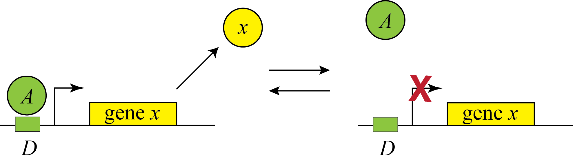
\begin{align} \beta(A) = \beta_0 \frac{D_\mathrm{occ}}{D_\mathrm{tot}} = \frac{\beta_0 A/K_\mathrm{d}}{1+A/K_\mathrm{d}}. \end{align}
This produces the opposite, mirror image response compared to repression, shown below with no leakage.
[4]:
A = np.linspace(0, 20, 200)
beta_A = A / (1 + A)
beta_R = 1 / (1 + R)

# Build plot
p = bokeh.plotting.figure(
    height=275,
    width=400,
    x_axis_label="A/Kd, R/Kd",
    y_axis_label="β/β₀",
    x_range=[R[0], R[-1]],
    y_range=[0, 1],
)

p.line(A, beta_A, line_width=2, legend_label="β(A)")
p.line(R, beta_R, line_width=2, color="tomato", legend_label="β(R)")
p.legend.location = "center_right"
bokeh.io.show(p)
Activator vs. Repressor–which to choose?
And now at last we have reached our first true ‘design’ question: The cell has at least two different ways to regulate a gene: using an activator or using a repressor. Which should it choose? Which would you choose if you were designing a synthetic circuit? Why? Are they completely equivalent ways to regulate a target gene? Is one better in some or all conditions? How could we know?
These questions were posed in a study by Michael Savageau (PNAS, 1974), and further developed in subsequent papers, to explain the naturally observed usage of activation and repression. A different explanation was later developed by Shinar et al (PNAS 2004). Try to think as a circuit designer about when and why you would employ one type of regulation or the other.
Computing environment
[5]:
%load_ext watermark
%watermark -v -p numpy,bokeh,jupyterlab
Python implementation: CPython
Python version       : 3.8.8
IPython version      : 7.21.0

numpy     : 1.19.2
bokeh     : 2.3.0
jupyterlab: 3.0.11