13. Bursty gene expression
Design principle
Bursty gene expression enables cells to regulate the mean and cell-cell variability of protein levels by controlling burst frequency and burst size.
Concepts
Master equations as gain-loss equations for probability.
Gene expression occurs in bursts.
Techniques
Manipulating master equations
Probability stories (Poisson, Geometric, and Negative Binomial)
In the last lesson, we laid out two objectives. First, we aimed to identify the sources of noise and how to characterize them. We summarized statistics about the probability distribution of copy numbers by considering the mean and coefficient of variation. The mean ends up following the same deterministic dynamics we have been considering thus far in the course. The coefficient of variation is a measure of noise, or relative departure from the mean behavior. Now, we will look at the dynamics of the entire probability distribution of copy number, \(P(n,t)\).
Master equations
We will use master equations to describe the dynamics of \(P(n,t)\). Generally, a master equation is a loss-gain equation for probabilities of states governed by a Markov process. In our case, the “state” is the set of copy numbers of molecular species of interest. The values of \(n\) are discrete, so we have a separate differential equation for each \(P(n,t)\). Specifically,
\begin{align} \frac{\mathrm{d}P(n,t)}{\mathrm{d}t} = \sum_{n'}\left[W(n\mid n') P(n',t) - W(n'\mid n)P(n,t)\right]. \end{align}
Here, \(W(n\mid n')\) is the transition probability per unit time of going from \(n'\) to \(n\).
The master equation makes sense by inspection and appears simple. The nuance lies in the definition of the transition rates, \(W(n\mid n')\). There is also the computational difficulty that \(n\) can be very large. In general, solving the master equation is difficult and is usually intractable analytically. Therefore, we sample out of the distribution. That is, we can draw many samples of values of \(n\) at time points \(t\) that are distributed according to the probability distribution that solves the master equation. We can then plot histograms to get an approximate plot of the probability distribution. We can also use the samples to compute moments, giving us estimates of the mean and variance. Generating the samples from the differential master equation is done using a Gillespie algorithm, also known as a stochastic simulation algorithm, or SSA. We will learn how to do these calculations in the next lesson.
The Master equation for unregulated gene expression
As we have seen, unregulated gene expression is described by the macroscale equation
\begin{align} \frac{\mathrm{d}n}{\mathrm{d}t} = \beta - \gamma n. \end{align}
To translate this into stochastic dynamics, we write the production rate as
\begin{align} \text{production rate} = \beta \delta_{n',n-1}, \end{align}
where we have used the Kronecker delta,
\begin{align} \delta_{ij} = \left\{\begin{array}{lll} 1 && i = j \\ 0 && i\ne j. \end{array} \right. \end{align}
This says that if our current copy number is \(n-1\), the probability that it moves to \(n\) in unit time is \(\beta\). Similarly, the decay rate is
\begin{align} \text{decay rate} = \gamma (n+1) \delta_{n',n+1}. \end{align}
This says that if we have \(n+1\) molecules, the probability that the copy number moves to \(n\) in unit time is \(\gamma(n+1)\). Thus, we have
\begin{align} W(n\mid n') = \beta \delta_{n',n-1} + \gamma (n+1)\delta_{n',n+1}. \end{align}
We can then write our master equation as
\begin{align} \frac{\mathrm{d}P(n,t)}{\mathrm{d}t} = \beta P(n-1,t) + \gamma(n+1)P(n+1,t) - \beta P(n,t) - \gamma n P(n,t), \end{align}
where we define \(P(n<0,t) = 0\).
This is a large set of ODEs, and as mentioned in the previous section, solving for \(P(n,t)\) is nontrivial and is usually done by Gillespie algorithm. Instead, let’s look for a steady state solution of this system of ODEs; i.e., let’s find \(P(n)\) that satisfies
\begin{align} \frac{\mathrm{d}P}{\mathrm{d}t} = 0. \end{align}
To solve this, we will start with the case where \(n=0\), noting that \(P(n<0) = 0\).
\begin{align} \gamma P(1) - \beta P(0) = 0 \;\;\Rightarrow P(1)\;\; = \frac{\beta}{\gamma}P(0). \end{align}
We can write the expression for the case where \(n=1\).
\begin{align} \beta P(0) + 2 \gamma P(2) - \beta P(1) - \gamma P(1) = 0 \;\;\Rightarrow\;\; P(2) = \frac{1}{2\gamma}\left(\beta P(1) + \gamma P(1) + \beta P(0)\right). \end{align}
We can use the fact that \(P(1) = \beta P(0) / \gamma\) to simplify this expression to
\begin{align} P(2) = \frac{1}{2}\left(\frac{\beta}{\gamma}\right)^2\,P(0). \end{align}
We do it again for \(n = 2\).
\begin{align} \beta P(1) + 3 \gamma P(3) - \beta P(2) - 2\gamma P(2) = 0 \;\;\Rightarrow\;\; P(3) = \frac{1}{3\gamma}\left(\beta P(2) - 2\gamma P(2) + \beta P(1)\right). \end{align}
Using our expressions for \(P(1)\) and \(P(2)\), we can rearrange this expression to write \(P(3)\) in terms of \(P(0)\), giving
\begin{align} P(3) = \frac{1}{6}\left(\frac{\beta}{\gamma}\right)^3\,P(0). \end{align}
We can continue this process over and over again such that for and \(n\), we have
\begin{align} P(n) = \frac{1}{n!}\left(\frac{\beta}{\gamma}\right)^n P(0). \end{align}
To solve for \(P(n)\), then, we need to find \(P(0)\) to do this, we can use the fact that the probability distribution must be normalized;
\begin{align} \sum_{n=0}^\infty P(n) = P(0) \sum_{n=0}^\infty \frac{1}{n!}\left(\frac{\beta}{\gamma}\right)^n = P(0)\mathrm{e}^{\beta/\gamma} = 1, \end{align}
where we have noted that the infinite sum is the Taylor series expansion of the exponential function. Thus, we have \(P(0) = \mathrm{e}^{-\beta/\gamma}\), and we have our steady state probability mass function,
\begin{align} P(n) = \frac{1}{n!}\left(\frac{\beta}{\gamma}\right)^n \mathrm{e}^{-\beta/\gamma}. \end{align}
We recognize this as the PMF of the Poisson distribution. We could perhaps have guessed this from the “story” of the Poisson distribution.
Rare events occur with a rate \(\lambda\) per unit time. There is no “memory” of previous events; i.e., that rate is independent of time. The probability that \(k\) events occur in unit time is Poisson distributed.
The story of mRNA production matches this story. The event here is the production of a gene product. We need these events to happen before decay. Apparently, the rate \(\lambda\) is in this case \(\beta/\gamma\).
It is useful also to consider the moments of the Poisson distribution and compute useful summary statistics of the distribution.
\begin{align} &\langle n \rangle = \frac{\beta}{\gamma}, \\[1em] &\langle n^2 \rangle - \langle n \rangle^2 = \sigma^2 = \frac{\beta}{\gamma}, \\[1em] &\text{noise} = \frac{\sigma}{\langle n \rangle} = \eta = \sqrt{\frac{\gamma}{\beta}}, \\[1em] &\text{Fano factor} = F = \frac{\sigma^2}{\langle n \rangle} = 1. \end{align}
Dynamics of the moments
From the master equation, we can derive an ODE describing the dynamics of the mean copy number of time, \(\langle n(t) \rangle\). To do this, we multiply both sides of the master equations by \(n\) and then sum over \(n\).
\begin{align} &\sum_{n=0}^\infty n \left[ \frac{\mathrm{d}P(n,t)}{\mathrm{d}t} = \beta P(n-1,t) + \gamma(n+1)P(n+1,t) - \beta P(n,t) - \gamma n P(n,t)\right] \nonumber \\[1em] &= \frac{d\langle n \rangle}{\mathrm{d}t} = \beta \sum_{n=0}^\infty n P(n-1,t) + \gamma \sum_{n=0}^\infty n(n+1)P(n+1,t) - \beta\langle n \rangle - \gamma \langle n^2 \rangle, \end{align}
where we have used the facts that
\begin{align} \langle n \rangle &= \sum_{n=0}^\infty n P(n,t), \\[1em] \langle n^2 \rangle &= \sum_{n=0}^\infty n^2 P(n,t). \end{align}
We have two sums left to evaluate.
\begin{align} \sum_{n=0}^\infty n P(n-1,t) = \sum_{n=0}^\infty (n+1)P(n,t) = \langle n \rangle + 1, \end{align}
and
\begin{align} \sum_{n=0}^\infty n(n+1)P(n+1,t) = \sum_{n=0}^\infty n(n-1)P(n,t) = \langle n^2 \rangle - \langle n\rangle. \end{align}
Thus, we have
\begin{align} \frac{d\langle n \rangle}{\mathrm{d}t} &= \beta(\langle n \rangle + 1) + \gamma (\langle n^2 \rangle - \langle n\rangle) - \beta\langle n \rangle - \gamma \langle n^2 \rangle \nonumber \\[1em] &= \beta - \gamma \langle n \rangle, \end{align}
which is precisely the macroscale ODE we are used to. It is now clear that it describes the mean of the full probability distribution.
Experimental Fano factors are greater than one
A nice feature of considering the whole probability distribution is that we can predict a value for the noise and Fano factor. Importantly, the Fano factor is invariant to parameters; it is always unity. So, if we see Fano factors of unity in experiment, we know our model for gene transcription is at least plausible.
Gene expression in individual cells typically results in a Fano factor greater than one! There are many ways this could come about, such as explicitly considering the multiple steps involved in making a protein, or by having a switchable promoter, as we will explore in the homework. Today, we will focus on a key experimental result: gene expression occurs in bursts.
Observations of bursty gene expression
In a beautiful set of experiments, Cai, Friedman, and Xie (Nature, 2006) discovered that gene expression is bursty. (We will come to understand what we mean by “bursty” in a moment.)
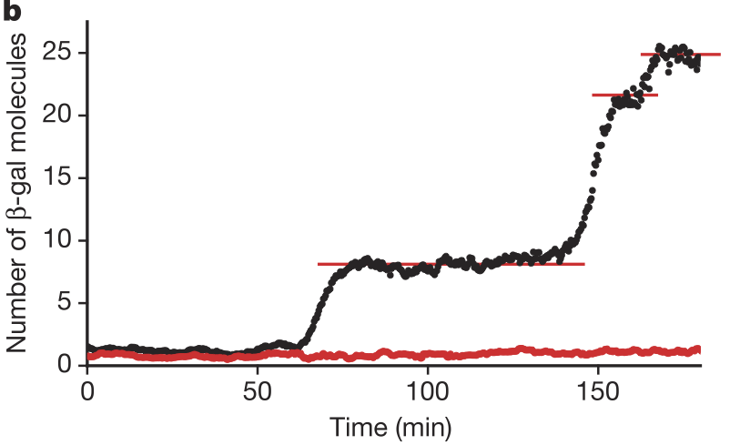
Through a clever experimental setup (I encourage you to read the paper), Cai, Friedman, and Xie were able to get accurate counts of the number of β-galactosidase molecules in individual cells over time. They found that the number of molecules was constant over long stretches of time, and then the number suddenly increased. The figure below, taken from the paper, shows the number of β-galactosidase molecules present in a single cell over time (black) and a blank background (red). This shows that expression of the β-gal gene happens in bursts. In each burst, many molecules are made, and then there is a period between bursts where no molecules are made.
Cai and coworkers also found that the number of molecules produced per burst was geometrically distributed, as shown in the figure below.
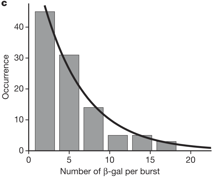
Recall, the “story” behind the Geometric distribution.
We perform a series of Bernoulli trials with success probability \(p_0\) until we get a success. We have \(k\) failures before the success. The probability distribution for \(k\) is Geometric.
The probability mass function for the Geometric distribution is
\begin{align} P(k;p_0) = (1-p_0)^k p. \end{align}
Considering this story, this implies that a burst is turned on, and then it turns off by a random process after some time.
Master equation for bursty gene expression
We also see from the experimental results tracking β-galactosidase copy number that the time scale of the bursty gene expression is much shorter than the typical decay time. So, per unit time, we can have many gene products made, not just a single gene product as we have considered thus far. So, we can re-write our transition probabilities per unit time as
\begin{align} W(n\mid n') &= \beta' \xi_{n-n'} - \gamma (n+1) \delta_{n+1,n'}, \end{align}
where \(\xi_{j}\) is the probability of making \(j\) molecules in a burst and \(\beta'\) is the probability per unit time of initiating production of molecules. If \(\xi_{j} = 0\) for all \(j\ne 1\), then \(\beta' = \beta\), and we have the same equations as before. So, our model is only slightly changed; we just allow for more transitions in and out of state \(n\).
We just have to specify \(\xi_{j}\). We know that the number of molecules produced per burst is geometrically distributed, so
\begin{align} \xi_j = p_0(1-p_0)^j. \end{align}
Now, our master equation is
\begin{align} \frac{\mathrm{d}P(n,t)}{\mathrm{d}t} &= \beta'\sum_{n'=0}^{n-1}p_0(1-p_0)^{n-n'} P(n',t) + \gamma(n+1)P(n+1,t) \nonumber \\[1em] &\;\;\;\;- \beta'\sum_{n'=n+1}^\infty p_0(1-p_0)^{n'-n}P(n,t) - \gamma n P(n,t). \end{align}
We can simplify the second sum by noting that it can be written as a geometric series,
\begin{align} \sum_{n'=n+1}^\infty p_0(1-p_0)^{n'-n} = p_0\sum_{j=1}^\infty (1-p_0)^j = p_0\left(\frac{1-p_0}{1-(1-p_0)}\right) = 1-p_0. \end{align}
Thus, we have,
\begin{align} \frac{\mathrm{d}P(n,t)}{\mathrm{d}t} &= \beta'\sum_{n'=0}^{n-1}p_0(1-p_0)^{n-n'} P(n',t) + \gamma(n+1)P(n+1,t) \nonumber \\[1em] &\;\;\;\;- \beta'(1-p_0)P(n,t) - \gamma n P(n,t). \end{align}
As we might expect, an analytical solution for this master equation is difficult. We are left to simulate it using SSA.
The steady state distribution for bursty expression is Negative Binomial
We could derive the steady state distribution of copy numbers under the bursty master equation, but we will instead take a story matching approach to guess the solution. The story of the Negative Binomial distribution is as follows.
We perform a series of Bernoulli trials with a success rate \(p_0\) until we get \(r\) successes. The number of failures, \(n\), before we get \(r\) successes is Negative Binomially distributed.
Bursty gene expression can give mRNA count distributions that are Negative Binomially distributed. Here, the Bernoulli trial is that a “failure” is production of and mRNA molecule and a “success” is that a burst in gene expression stops. So, the parameter \(p_0\) is related to the length of a burst in expression (lower \(p_0\) means a longer burst). The parameter \(r\) is related to the frequency of the bursts. If multiple bursts are possible within the lifetime of mRNA, then \(r > 1\). Then, the number of “failures” is the number of mRNA transcripts that are made in the characteristic lifetime of mRNA.
The Negative Binomial distribution is equivalent to the sum of \(r\) Geometric distributions. So, the number of copies will be given by how many bursts we get before degradation. This suggests that \(r = \beta'/\gamma\). We can then write the Negative Binomial probability mass function as
\begin{align} P(n;r,p_0) = \frac{(n+r-1)!}{n!(r-1)!} p_0^r(1-p_0)^n, \end{align}
where \(r = \beta'/\gamma\). You can plug this in to the master equation to verify that this is indeed a steady state.
We can put this in more convenient form. Instead of using \(p_0\) to parametrize the distribution, we can instead define the burst size \(b\) as the mean of the geometric distribution describing the number transcripts in a burst,
\begin{align} b = \frac{1-p_0}{p_0}. \end{align}
Recall that \(r\) is the typical number of bursts before degradation (or dilution), so \(r\) is a burst frequency. So, for convenience, we write the steady state distribution as
\begin{align} P(n;r,b) = \frac{(n+r-1)!}{n!(r-1)!}\,\frac{b^n}{(1+b)^{n+r}}. \end{align}
Strictly speaking, \(r\) can be non-integer, so
\begin{align} P(n;r,b) = \frac{\Gamma(n+r)}{n!\Gamma(r)!}\,\frac{b^n}{(1+b)^{n+r}}, \end{align}
where \(\Gamma(x)\) is the gamma function.
The Negative Binomial is interesting because it can be peaked for \(r > 1\), but has a maximum at \(n=0\) for \(r < 1\). So, for a low burst frequency, we get several cells with zero copies, but we can also get cells with many. This might have interesting implications on the response of a group of cells to a rise in lactose concentration and also drop in other food sources. If \(r < 1\), we then have a simple explanation for the “all-or-none” phenomenon of induction observed 60 years ago in E. coli by Novick and Weiner (PNAS, 1957). Cells are either fully induced or not at all; with \(r < 1\), many cells have no \(\beta\)-galactosidase at all.
The known summary statistics of the negative binomial distribution are also useful.
\begin{align} \langle n \rangle &= rb \\[1em] \langle n^2 \rangle &= rb(1+b+rb) \\[1em] \sigma^2 &= rb(1+b) \\[1em] \text{Fano factor} = F &= 1+b \\[1em] \text{noise} = \eta &= \sqrt{\frac{1+b}{rb}}. \end{align}
So, we can tune the burst frequency and burst size to control variability. For example, we could keep \(\langle n \rangle\) constant by increasing the burst size \(b\) while decreasing the burst frequency \(r\) (big, intermittent bursts), which would result in increased noise. If, instead, we decreased the burst size while increasing the burst frequency (short, frequent bursts), we get reduced noise. This gives a design principle, bursty gene expression enables cells to regulate the mean and cell-to-cell variability of protein levels by controlling burst frequency and burst size.