6. Incoherent feed-forward loops generate pulses, speed responses, and serve as dosage compensators
Development of the sections of this chapter on dosage compensation benefited greatly from discussions with Michael Flynn.
Design principles
The I1-FFL with AND logic is a pulse generator and also speeds response compared to an unregulated circuit.
The incoherent feed-forward loop allows dosage-compensated gene expression.
[1]:
# Colab setup ------------------
import os, sys, subprocess
if "google.colab" in sys.modules:
    cmd = "pip install --upgrade colorcet biocircuits watermark"
    process = subprocess.Popen(cmd.split(), stdout=subprocess.PIPE, stderr=subprocess.PIPE)
    stdout, stderr = process.communicate()
# ------------------------------
import numpy as np
import scipy.integrate

import biocircuits.apps

import bokeh.io
import bokeh.layouts
import bokeh.models
import bokeh.plotting

import colorcet
colors = colorcet.b_glasbey_category10

bokeh.io.output_notebook()
In the previous chapter, we found that two of the eight architectures of feedforward loops were overrepresented in E. coli and S. cerevisiae, the C1-FFL and the I1-FFL. We analyzed the C1-FFL in detail, in so doing laid the groundwork for analyzing feedforward loops in genetic circuits in general. In this chapter, we turn our attention to the other over-represented circuit, the I1-FFL. As a reminder, here is the structure of the circuit.
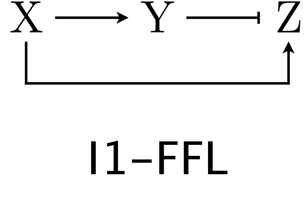
X activates Y and Z, but Y represses Z. We can use the expressions for production rate under AND and OR logic for one activator/one repressor that we showed above in writing down our dynamical equations. Here, we will consider AND logic. The dimensionless dynamical equations are
\begin{align} \frac{\mathrm{d}y}{\mathrm{d}t} &= \beta\,\frac{(\kappa x)^{n_{xy}}}{1+(\kappa x)^{n_{xy}}} - y,\\[1em] \gamma^{-1}\,\frac{\mathrm{d}z}{\mathrm{d}t} &= \frac{x^{n_{xz}}}{(1 + x^{n_{xz}})\,(1 + y^{n_{yz}})} - z. \end{align}
The I1-FFL with AND logic is a pulse generator
In our first analysis of this circuit, we will investigate the response in Z to a sudden, sustained step in stimulus X. We will choose \(\gamma = 10\), which means that the dynamics of Z are faster than Y.
(To solve and plot the dynamics, we will use the plot_ffl() function of the FFL app in the biocircuits package. This is essentially the same as the plot_ffl() function we coded up in the previous lesson, except it also returns some ColumnDataSources for the app, which we will ignore here.)
[2]:
# Parameter values
beta = 5
gamma = 10
kappa = 1
n_xy, n_yz = 3, 3
n_xz = 5
t = np.linspace(0, 10, 200)

# Set up and solve
p, _, _ = biocircuits.apps.plot_ffl(
    beta,
    gamma,
    kappa,
    n_xy,
    n_xz,
    n_yz,
    ffl="i1",
    logic="and",
    t=t,
    t_step_down=np.inf,
    normalized=False,
)
bokeh.io.show(p)
We see that Z pulses up and then falls down to its steady state value. This is because the presence X leads to production of Z due to its activation. X also leads to the increase in Y, and once enough Y is present, it can start to repress Z. This brings the Z level back down toward a new steady state where the production rate of Z is a balance between activation by X and repression by Y. Thus, the I1-FFL with AND logic is a pulse generator.
The I1-FFL with AND logic gives an accelerated response
Let us compare the response of an I1-FFL being suddenly turned on (by a step in X) to an unregulated circuit that achieves the same steady state. Recall that the dimensionless dynamics for the unregulated circuit (that is, X ⟶ Z, the circuit in the absence of Y) follow
\begin{align} z(t) = 1 - \mathrm{e}^{-t}, \end{align}
as derived in the chapter on small circuits.
If we plot the normalized I1-FFL together with the unregulated response, we see that the I1-FFl makes it to the steady state faster, though it overshoots and then relaxes.
[3]:
p, _, _ = biocircuits.apps.plot_ffl(
    beta,
    gamma,
    kappa,
    n_xy,
    n_xz,
    n_yz,
    ffl="i1",
    logic="and",
    t=t,
    t_step_down=np.inf,
    normalized=True,
)

# Unregulated dynamics
p.line(
    t, 1 - np.exp(-t), line_width=2, color=colors[4], legend_label="unregulated",
)

bokeh.io.show(p)
So, we have another design principle, The I1-FFL with AND logic has a faster response time than an unregulated circuit.
The accelerated response of the I1-FFL is observed experimentally
Mangan and coworkers (J. Molec. Biol., 2006) investigated an I1-FFL circuit that E. coli uses in its galactose utilization system. The circuit is shown below.

As the “X” gene in this I1-FFL is CRP, the circuit is induced by sudden addition of cAMP, as in the arabidose and lactose circuits above. Mangan and coworkers investigated the response of the wild type circuit, as well as a mutant circuit where galS was deleted. This latter circuit lacks the feed forward loop, and the production of galETK is directly regulated by CRP.
In their experiment, the galE promoter was engineering to express GFP so they could monitor the dynamics of the circuit with fluorescence. The result is shown below.
[4]:
# Plot data digitized from Mangan, et al., J. Molec. Biol., 2006
# https://doi.org/10.1016/j.jmb.2005.12.003

t_wt = np.array([
    0.07, 0.39, 0.71, 0.94, 1.2 , 1.45, 1.67, 1.9 , 2.14, 2.35, 2.55,
    2.74, 2.89, 3.05])

t_mut = np.array([
    0.05, 0.29, 0.58, 0.83, 1.05, 1.28, 1.53, 1.75, 1.96, 2.17, 2.37])

x_wt = np.array([
    0.04, 0.56, 1.11, 1.53, 1.73, 1.78, 1.67, 1.44, 1.3 , 1.2 , 1.11,
    1.05, 1.  , 1.  ])

x_mut = np.array([
    0.04, 0.16, 0.32, 0.46, 0.5 , 0.56, 0.62, 0.68, 0.71, 0.75, 0.79])

p = bokeh.plotting.figure(
    frame_height=250,
    frame_width=350,
    x_axis_label='time (cell divisions)',
    y_axis_label="normalized level",
)

p.circle(t_wt, x_wt, color=colors[0], legend_label="wild type")
p.circle(t_mut, x_mut, color=colors[1], legend_label="galS mutant")

p.legend.location = "bottom_right"

bokeh.io.show(p)
We see that indeed the wild type I1-FFL architecture speeds up the response to the cAMP input, complete with the overshoot we expect from an I1-FFL circuit.
Gene dosage varies in bacteria
One of the most intriguing functions of an I1-FFL is its ability to address the problem of gene dosage compensation.
Consider a gene, x, whose protein product, p, is needed at a particular concentration in the cell. Previously, we saw that if the gene is expressed at a constitutive rate, \(\beta\), and removed with rate constant \(\gamma\), its steady-state concentration will be \(p_{st}=\beta/\gamma\).
However, this treatment neglected an important variable in the system: gene dosage, defined as the number of DNA copies of that gene. We tend to think of gene dosage as a fairly stable number, but in fact it can vary a lot across different cellular contexts. For example, in rich media, bacteria have the remarkable ability to divide with a cell cycle time that is shorter than the time required to replicate their own chromosome. This seemingly paradoxical feat is achieved through concurrent replication processes, also known as “dichotomous replication.” The cell initiates a round of chromosomal replication. But it’s in a hurry, so before that round is complete, it initiates a new round, and so. on. As a result, depending on where a gene is located on the chromosome, and where the cell is in the cell cycle, the gene may exist in 1,2,4, or potentially even more copies.
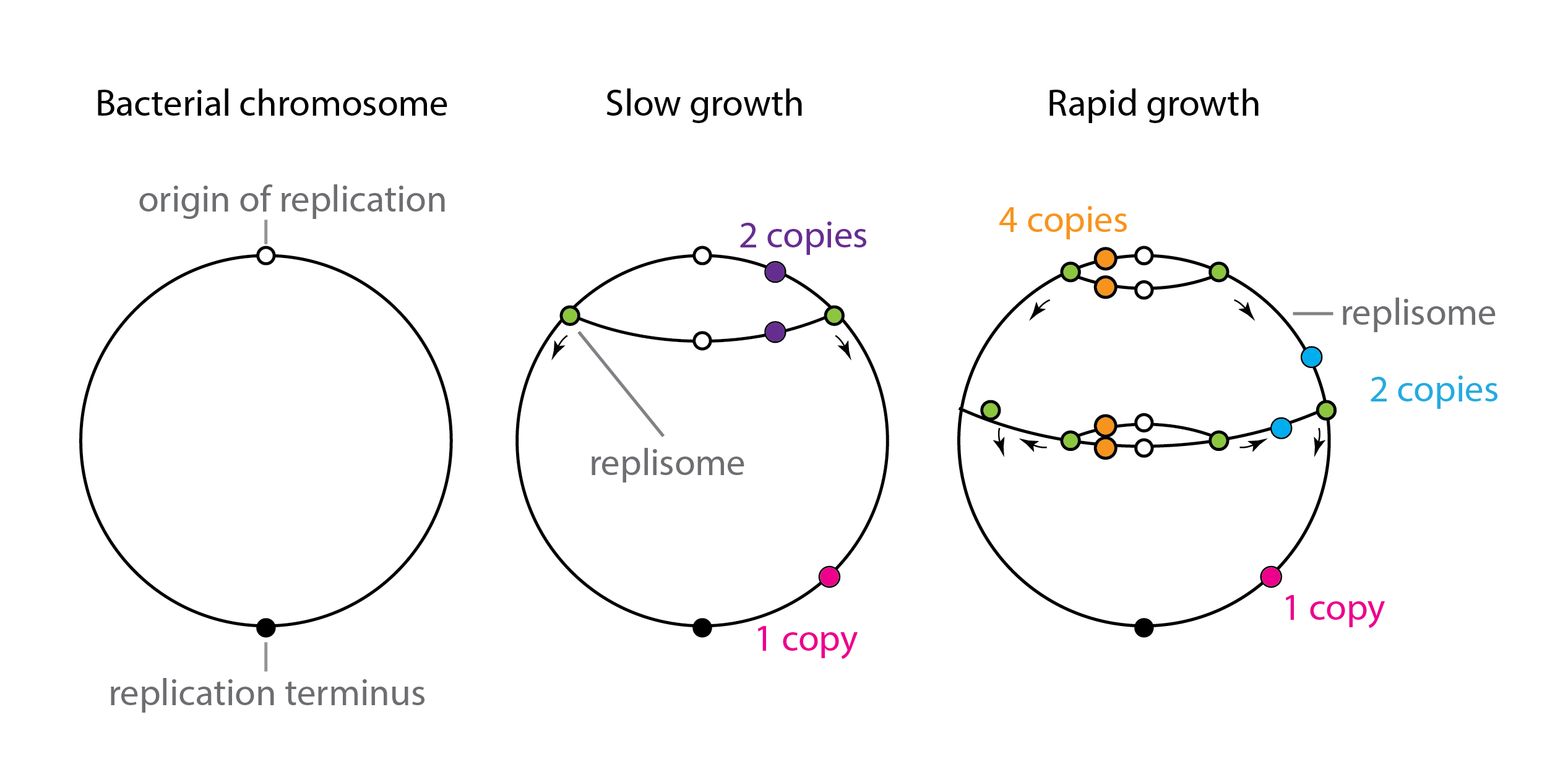
Schematic view of dichotomous replication, after similar diagram in Trojanowski et al,Front. Microbiol. 2018
In addition to this level of dosage variation, plasmids (self-replicating circular DNA molecules) in bacteria can exist at a widely varying range of copy numbers depending on growth conditions, and can be transferred (in some cases) laterally from one cell to another. Thus, genes on a plasmid may also need mechanisms to compensate for variations in their own dosage.
Gene dosage also varies in eukaryotic cells
Eukaryotic cells also experience another form of gene dosage variation: changes in ploidy. For instance, chromosome numbers double in the G2 phase (after replication) compared to G1 (before replication). Ploidy can also vary in other contexts. Muscle, liver, heart, bone marrow, and placenta all contain polyploid cells with multiple copies of chromosomes. In these cases, the copy number of the whole genome is altered in the same proportion. And sometimes this comes along with an increase in total cell volume.
Sex chromosomes can be present at different numbers in males and females, leading to variation in gene dosage. For example, in humans, the X chromosome exists at one copy per cell in males but two in females. This is solved through randomly silencing, or “inactivating,” one of the two X chromosomes in each cell. (The “calico” coat pattern in cats is partly explained by mosaic clones in which different X chromosomes, carrying coat color genes, are inactivated this way.) In Drosophila, males increase expression of genes on their one X chromosome by two-fold. In C. elegans, hermaphrodites, with two X chromosomes, do the opposite, down-regulating the expression of each X by 50% to match the X expression in males, which contain only one X chromosome.
In cancer, certain chromosomal regions can be duplicated multiple times, amplifying their copy number. These amplifications can drive cancer cell survival and replication. This is a different, aberrant, context in which gene dosage can similarly vary.
Gene dosage compensation is important for synthetic biology and gene therapy applications.
In synthetic biology and metabolic engineering, there is great interest in designing genetic systems that can operate predictably across different contexts, despite all of this dosage variation.
Gene therapies seek to provide cells with a replacement copy of a gene that is otherwise mutated or inactivated in the patient. This gene could be inserted into cells in different ways. One currently popular approach uses adeno-associated virus (AAV) vectors, which can efficiently enter cells and allow expression of their DNA cargo. With these systems, it is impossible to precisely control the number of copies of the gene that are delivered to each cell—some cells may receive many copies, while others receive fewer, or none. Furthermore, with vectors that integrate in the genome, the precise location of integration can influence the level of expression of the gene. As a result, even if each cell received the same number of copies, those copies might express at different levels in different cells. Thus, without some mechanism to compensate for dosage variation, the gene therapy will be expressed at a range of different levels in different cells.
In fact, if merely providing the protein at any level were sufficient, this variability might be tolerable. However, in some cases too much of the “good” protein can be almost as bad as too little. One example of this “Goldilocks” problem occurs in Rett syndrome, a devastating condition that results from loss of function of the gene MeCP2, which is on the X chromosome. In heterozygous females, half of cells express mutant MeCP2, leading to disease. Yet overexpression of MeCP2 is also toxic, leading to a condition known as MeCP2 duplication syndrome. For these reasons, gene dosage compensation could be important for gene therapy as well as for endogenous organismal regulation.
The transcriptional IFFL can provide gene dosage compensation
Recent work has shown that the incoherent feed-forward loop (IFFL) can provide a remarkably simple mechanism for gene dosage compensation. Here, we will explore two different IFFL designs that use either transcriptional or post-transcriptional (micro-RNA) regulation in bacteria or mammalian cells, respectively.
We start with a beautiful demonstration of dosage compensation in bacteria by Segall-Shapiro, Sontag, and Voigt (2018). The authors described a synthetic system that reduces the sensitivity of the concentration of an expressed protein to variation in the copy number of its gene. Consider our usual gene expression system, except we now explicitly include the gene copy number, denoted \(C\), as a parameter. Assuming the gene copies are independent of one another and otherwise identical, the dynamics of our constitutively expressed gene can be written,
\begin{align} \frac{\mathrm{d}y}{\mathrm{d}t} = \beta C - \gamma y \end{align}
Where Y is our protein of interest, \(\beta\) is the production rate from each copy of the gene and \(\gamma\) is the degradtion rate, as before. The steady-state value of Y, denoted \(Y_\mathrm{ss}\), is then
\begin{align} Y_\mathrm{ss} = \frac{\beta C}{\gamma} \end{align}
\(Y_\mathrm{ss}\) is linearly dependent on the copy number of the gene, as we would expect for this simple system.
Now consider what happens when we make the system a little more interesting. Suppose we add a repressor, X, that can repress expression of Y. Further, suppose X and Y are encoded in adjacent (but independently expressed) genes, and therefore share the same copy number within the cell. This type of arrangement produces a kind of IFFL, in which gene copy number controls expression of both X and Y, and the product of X further represses expression of Y.

To see how the IFFL affects steady state Y expression, we start by writing down ODEs for X and Y in the IFFL system. We allow each gene to have a distinct transcription rate, either \(\beta_x\) or \(\beta_y\), respectively, and the same Hill-type repression that we have considered previously. For simplicity, we will assume that X and Y have the same effective degradation rate: \(\gamma_x = \gamma_y = \gamma\).
\begin{align} \frac{\mathrm{d}x}{\mathrm{d}t} &= \beta_x C - \gamma x \\ \frac{\mathrm{d}y}{\mathrm{d}t} &= \frac{\beta_yC}{1 + \left(\frac{x}{k}\right)^n} - \gamma y \end{align}
Non-dimensionalizing, we obtain:
\begin{align} \frac{\mathrm{d}x}{\mathrm{d}t} &= \beta \, C - x, \\[1em] \frac{\mathrm{d}y}{\mathrm{d}t} &= \frac{C}{1 + x^n} - y, \end{align}
where we have nondimensionalized \(x\) and \(y\) according to \(x \leftarrow x/k\) and \(y \leftarrow y/(\beta_y/\gamma)\) and defined \(\beta = \beta_x / k \gamma\).
Solving for steady states, we obtain:
\begin{align} x_\mathrm{ss} &= \beta C \\ y_\mathrm{ss} &= \frac{C}{1 + (\beta C)^n} \end{align}
In the limit of large enough \(C\),
\begin{align} y_\mathrm{ss} \approx \frac{C}{(\beta C)^n}. \end{align}
When \(n=1\), this is just \(y_\mathrm{ss} = 1/\beta\). In other words, when \(n=1\), the expression of \(Y\) becomes independent of copy number, as desired. Further, \(n=1\) is not an unrealistic assumption. In fact, many prokaryotic gene regulation systems exhibit simple linear repression.
We see that as long as the copy number is high enough, the IFFL makes steady state expression of Y independent of copy number \(C\). What a remarkable thing. Just by adding one additional regulator, changes in gene dosage can be compensated out!
One might, however, still ask how sensitive this capability is to the Hill coefficient of repression. Does it require \(n=1\)? We can plot the steady state dimensionless Y concentration, allowing for varying \(\beta\) and \(n\).
[5]:
# Initial parameters on plot
beta = 1
n = 1

# Build plot
p = bokeh.plotting.figure(
    frame_width=300,
    frame_height=150,
    x_axis_label="copy number",
    y_axis_label="dimensionless yₛₛ",
)

# Plot unregulated case
C = np.arange(201)
y = C / (1 + (beta * C) ** n)
cds = bokeh.models.ColumnDataSource(dict(C=C, y=y))
p.circle(source=cds, x="C", y="y")

# Sliders for controlling parameters
beta_slider = bokeh.models.Slider(
    title="β",
    start=-1,
    end=1,
    step=0.1,
    value=0,
    width=150,
    format=bokeh.models.FuncTickFormatter(code="return Math.pow(10, tick).toFixed(2)"),
)

n_slider = bokeh.models.Slider(
    title="n", start=0.1, end=4, step=0.1, value=1, width=150
)

# JavaScript code for callback
js_code = """
// Extract data from source and sliders
let C = cds.data['C'];
let y = cds.data['y'];
let beta = Math.pow(10, beta_slider.value);
let n = n_slider.value;
// Update steady state levels
for (let i = 0; i < C.length; i++) {
    y[i] = C[i] / (1 + Math.pow(beta * C[i], n));
}
// Emit changes
cds.change.emit();
"""

callback = bokeh.models.CustomJS(
    args=dict(cds=cds, beta_slider=beta_slider, n_slider=n_slider), code=js_code
)

# Link callback
beta_slider.js_on_change("value", callback)
n_slider.js_on_change("value", callback)

# Build layout
layout = bokeh.layouts.row(
    p, bokeh.layouts.Spacer(width=30), bokeh.layouts.column(beta_slider, n_slider)
)
bokeh.io.show(layout)
In fact, it does. We can see that \(n=1\) generates ideal dosage-independent behavior. With \(n > 1\), \(y_\mathrm{ss}\) responds non-monotonically to copy number, producing a peak in Y concentration at intermediate copy numbers. By contrast, if \(n < 1\), we observe an attenuated incomplete dosage compensation. For bacteria, we are fortunate (for this circuit) that gene regulation can be linearly sensitive (\(n=1\)) in many cases.
Synthetic biology enables experimental tests of dosage compensation in bacteria
To test the bold prediction that the IFFL can dosage compensate expression, Voigt and colleagues designed a synthetic gene regulatory system incorporating a variety of designed regulatory elements. As a repressor, they used Transcription activator-like effector (TALE) proteins derived from Xanthamonas bacteria that infect plants. These proteins exhibit a programmable structure based on modular ≈34 amino acid units that recognize different DNA dinucleotides. By concatenating these modules, one can design TALE proteins that target desired DNA binding sites. Just prior to the emergence of CRISPR as powerful and versatile programmable gene editing system, TALEs were poised to provide many similar functions. For the purposes of this experiment, key properties of the TALE repressors include their ability to tightly (≈100-fold) repress target promoters in bacteria and their ability, demonstrated in this paper, to provide linearly sensitive (\(n=1\)) repression. To control the copy number, the authors expressed each system from a series of plasmids with different copy numbers. The following plot from their paper demonstrates the remarkable ability of this system to eliminate dosage-dependence.
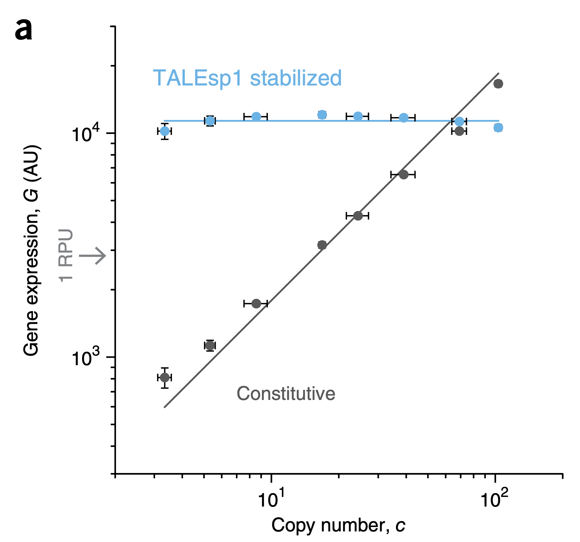
Figure fromSegall-Shapiro et al, Nat. Biotech., 2018. An unregulated promoter, black, exhibits linear sensitivity to dosage. By contrast, the IFFL system, blue, produces dosage-independent gene regulation across a broad range of copy numbers. Each system was expressed from a set of different plasmids exhibiting varying copy numbers.
While expression could be made independent of gene copy number, it could still be tuned by using promoters of different strengths. This corresponds to varying \(\beta_y\) in the equations above:
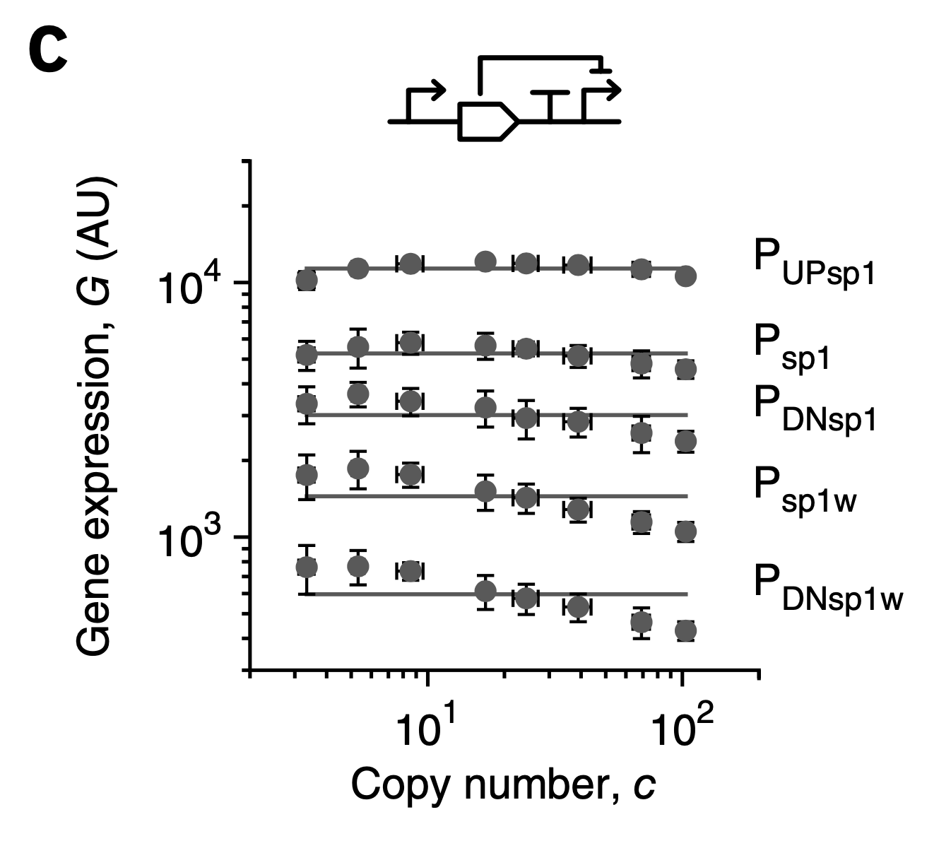
Figure fromSegall-Shapiro et al, Nat. Biotech., 2018. Different promoters allow different strengths of dosage-compensated expression.
Segall-Shapiro et al conclude: > This project started with a simple question. Could we design a promoter that produces the same protein concentration no matter where it is placed? Based on a simple model, we were able to design a class of stabilized promoter that maintained the same level of gene expression irrespective of the plasmid backbone or its location in the genome. This was achieved by harnessing the feedforward loop, a common motif in natural regulatory networks that is responsible for maintaining homeostasis between proteins, implementing dynamic ordering and producing a pulse of gene expression. Although our stabilized promoter was designed to buffer gene expression against the effects of changing DNA copy number, our results demonstrated broad robustness of the promoter design to genome mutations and medium composition. Collectively, robustness to these conditions eliminates much of the context dependence that plagues precision genetic engineering.
Single-gene miRNA-based IFFLs provide dosage compensation in mammalian cells
The strategy above appears to provide nearly ideal dosage compensation in bacteria. But several features make it unsuitable for mammalian gene therapies. For one thing, TALEs are large genes that take up a lot of the limited real estate of gene therapy vectors such as AAVs. Another issues is that it is generally more difficult in mammalian cells to isolate adjacent genes. A constitutive “\(X\)” could lead to undesired expression of an adjacent target gene, \(Y\). Finally, in a mammalian cell, gene regulation can be bursty (as we shall see soon in this course) and there can be delays of many hours for the transcription and translation of the constitutively expressed repressor, potentially leading to pulses and other dynamic behaviors.
In 2011, Kobe Benenson and colleagues published a paper entitled, “Synthetic incoherent feedforward circuits show adaptation to the amount of their genetic template”, which examined several different IFFL designs in mammalian cells. Two of their circuits used microRNA (miRNA) to post-transcriptionally implement the inhibition of Y by X. The most compact circuit is shown here:
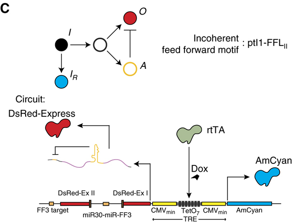
Image fromBleris et al, Molecular Systems Biology, 2011
In this simple circuit, the small molecule doxycycline (dox) can be used to induce expression of two divergently oriented genes. Dox binds to the reverse tet trans-activator protein (rtTA), allowing it to bind to a casette of 7 binding sites. Once bound, it activates expression of cyan and red fluorescent proteins. The two fluorescent proteins differ, however, in a crucial way: The protein coding sequence of the red protein is interrupted by an intron, an element that is removed in the nucleus through a process called splicing. Within the element is a micro-RNA that can be further processed and integrated into a complex called RISC which can specifically target and repress expression of the spliced mRNA in the cytoplasm via a target site in its 3’ untranslated region (UTR). This design thus constitutes a single gene I1-FFL!
In this astonishingly compact unit, increasing gene copy number should produce more mRNA encoding the red fluorescent protein as well as more miRNA to repress it. Does this design produce dosage compensation?
Addressing this question rigorously would require analyzing the various steps of splicing and processing of the miRNA. For simplicity here, we will consider a simplified model that suggests dosage compensation might be possible.
Because the relevant dynamics occur at the RNA level, we will change notation slightly. We will assume that the processed miRNA in its active RISC complex, denoted \(r\), is produced at a rate proportional to gene dosage, \(C\), and is degraded at a constant rate, \(\gamma_r\). Similarly, we assume the mRNA, denoted \(m\), is also produced at a rate proportional to copy number. In general, the production rates for the two species can differ, since producing mature mRNA and producing a mature RISC-miRNA complex involve distinct steps. We further assume that miRNA and mRNA interact at a rate governed by mass action kinetics, i.e. proportional to \(r \times m\) , with rate constant k, and that this interaction enzymatically destroys \(m\) but does not affect \(r\). Finally, we assume that the mRNA can degrade with a rate constant \(m\). With these assumptions, we can write down ordinary differential equations for the system.
\begin{align} \frac{\mathrm{d}r}{\mathrm{d}t} &= \beta_r C - \gamma_r r, \\[1em] \frac{\mathrm{d}m}{\mathrm{d}t} &= \beta_m C - k \,r \,m - \gamma_m m. \end{align}
To nondimensionalize, we set: - \(\tilde{t} = \gamma_r t\). This rescales time in units of the RISC lifetime. - \(\tilde{r} = r/(\beta_r/\gamma_r)\). This effectively normalizes \(r\) by its unregulated steady-state value for single copy expression. - \(\tilde{m} = m/(\beta_m/\gamma_m)\). This similarly normalizes \(m\). - \(\gamma = \gamma_m/\gamma_r\) and \(\kappa = \beta_r k/\gamma_r \gamma_m\). These represent the key dimensionless parameter ratios that will be important later.
\begin{align} \frac{\mathrm{d}\tilde{r}}{\mathrm{d}\tilde{t}} &= C - \tilde{r}, \\[1em] \gamma^{-1}\,\frac{\mathrm{d}\tilde{m}}{\mathrm{d}\tilde{t}} &= C - \kappa \,\tilde{r} \,\tilde{m} - \tilde{m}. \end{align}
At steady state, the time derivatives vanish, and we have
\begin{align} &C - \tilde{r}_\mathrm{ss} = 0 \\[1em] &C - \kappa\, \tilde{r}_\mathrm{ss}\, \tilde{m}_\mathrm{ss} - \tilde{m}_\mathrm{ss} = 0, \end{align}
which is readily solved to give
\begin{align} &\tilde{r}_\mathrm{ss} = C \\[1em] &\tilde{m}_\mathrm{ss} = \frac{C}{1 + \kappa C}. \end{align}
This is the same functional form as we saw in the synthetic I1-FFL E. coli dosage compensation circuit. In the regime where \(\kappa C \gg 1\), the steady state mRNA level becomes independent of copy number. To understand what this means in terms of requirements of the circuit function, let us write \(\kappa C\) in an instructive way. We know that the dimensional steady state concentration of active RISC complex is
\begin{align} r_\mathrm{ss} = \frac{\beta_r C}{\gamma_r}. \end{align}
Let \(m_\mathrm{ss}\) be the dimensional steady state concentration of mRNA. Then, the ratio of RISC-dependent to RISC-independent degradation of mRNA is
\begin{align} \frac{\text{rate of degradation by RISC}}{\text{rate of unassisted degradation}} = \frac{k\,r_\mathrm{ss}\,m_\mathrm{ss}}{\gamma_m m_\mathrm{ss}} = \frac{k \beta_r C/\gamma_r}{\gamma_m} = \kappa C. \end{align}
So, in order to have dosage independence, we need fast degradation by RISC relative to unassisted degradation or dilution. This is accomplished by having high copy number (thereby producing a lot of RISC), a fast production rate of RISC (high \(\beta_r\)), fast kinetics of degradation by RISC (high \(k\)), slow degradation of RISC (low \(\gamma_m\)), and slow unassisted degradation of mRNA (low \(\gamma_m\)).
The dimensional steady state of mRNA concentration is, in the limit of \(\kappa C \gg 1\),
\begin{align} m_\mathrm{ss} = \frac{\beta_m}{\gamma_m}\,\frac{C}{1+\kappa C} \approx \frac{\beta_m}{\kappa\,\gamma_m} = \frac{\beta_m\gamma_r}{\beta_r k}. \end{align}
Importantly, the copy number of mRNA can by tuned by adjusting the production rate of mRNA, \(\beta_m\) without destroying the copy-number-independence of the mRNA levels.
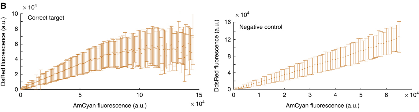
The following plots, from Bleris et al, 2011, show that in an unregulated system, the two fluorescent proteins would exhibit a linear relationship (right). but with the miRNA IFFL, the regulated red fluorescent target approaches a saturating value at higher levels of expression. (The dynamic range of expression levels is modest here—exploring a broader range would help to reveal the full behavior of this system). These data suggest that dosage compensation can be achieved with a single, post-transcriptionally self-regulating gene implementing a variant of the I1-IFFL motif.
Conclusions
The incoherent feed-forward loop is as mysterious as it is prevalent. Why would one want to regulate the same target gene in two opposite ways? The examples above suggest a few of its many dynamic functions: generating adaptive responses to step increases in input, accelerating responses, and, perhaps most dramatically, making gene expression independent of the dosage of the gene itself. IFFLs have also been shown to play other, related, roles as well, such as implementing fold-change detection, which occurs in systems whose outputs depend only on the fold increase of their inputs, irrespective of their absolute values.
Computing environment
[6]:
%load_ext watermark
%watermark -v -p numpy,scipy,bokeh,colorcet,biocircuits,jupyterlab
Python implementation: CPython
Python version       : 3.8.8
IPython version      : 7.22.0

numpy      : 1.20.1
scipy      : 1.6.2
bokeh      : 2.3.1
colorcet   : 2.0.6
biocircuits: 0.1.3
jupyterlab : 3.0.14