12. Gene expression is noisy! How stochastic effects lead to heterogeneity
Concepts
Intrinsic and extrinsic noise
Techniques
Plug-in estimates
Pairs bootstrap
Generative Bayesian modeling
[1]:
# Colab setup ------------------
import os, sys
if "google.colab" in sys.modules:
    data_path = "https://biocircuits.github.io/chapters/data/"
else:
    data_path = "data/"
# ------------------------------

import numpy as np
import pandas as pd

import bokeh.models
import bokeh.plotting
import bokeh.io

bokeh.io.output_notebook()
Thus far, we have written deterministic systems of ordinary differential equations to describe the dynamics of mRNA and protein concentrations in cells. These expressions assume that there are enough of all the components, and enough time, to sample all of the many available molecular states. So, we were looking at rates of gene expression considering large numbers of the molecular constituents. However, as we will see in the next two chapters, within a cell, biochemical processes can be quite stochastic (a term meaning intrinsically random) or “noisy.”
Over the next chapters we will focus on understanding the sources and dynamics of noise, methods to analyze noise, and the functional roles of noise in biological systems. To do so, we will use the mathematical machinery of probability, an important tool for every biologist and bioengineer to have in their toolbox.
Noise is present in genetic circuits, and cells are like burritos
One cell may seem at first glance identical to any other cell living alongside it in the same conditions. However, the inside of cells are heterogeneous and may be highly variable. Furthermore, the copy numbers of many proteins and mRNA molecules are small in a given cell. Wi and coworkers (Cell, 2014) used ribosome profiling to obtain estimates for absolute protein counts of various transcription factors. They found that half of repressors have copy numbers below 100 per genome equivalent and 90% of activators do as well. About 10% of repressors and 50% of activators have copy numbers of 10 or below. These are small numbers! This means that they are susceptible to fluctuations.
Generally speaking, we call deviations from what we might expect from our deterministic view of gene expression stochasticity, or noise. This is a key concept, because nearly all cellular processes are susceptible to noise for a host of reasons, especially low copy numbers of molecular regulators of gene expression. We will provide a more careful definition of noise momentarily.
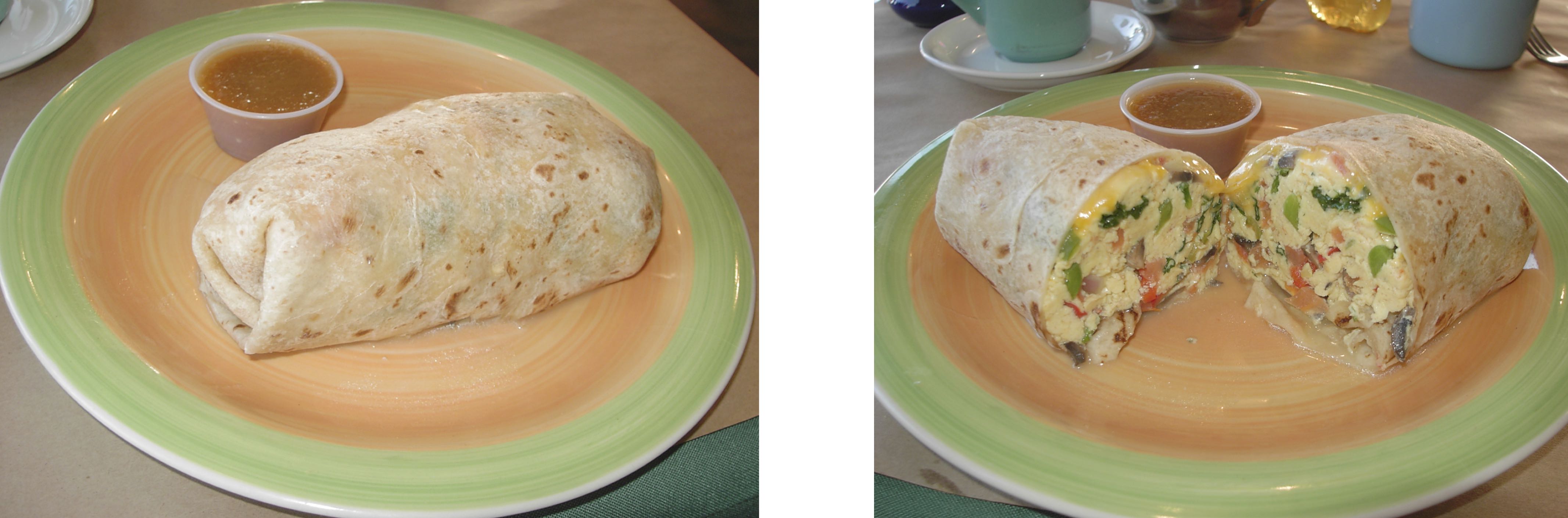
Consider the model of an E. coli cell depicted below. From the outside (left image), it appears as a simple cylindrical container, encapsulating what one might incorrectly assume is a homogeneous well-mixed continuum of biochemical mush inside. However, if we were to slice open the cell (right image), the low copy numbers of certain molecules and their spatial heterogenetiy become apparent. Within each cell, the copy numbers and locations of different molecules can vary dramatically over time, just as they vary from cell to cell. Like burritos, no two are truly identical. (Unlike this burrito, most bacteria do not include cheese in the periplasm.)
Looking at heterogeneity
To demonstrate the heterogeneity that may arise from small copy numbers, Boris Rotman (PNAS, 1961) performed a classic experiment in which he put small numbers (on average one) of β-D-galactosidase in droplets containing a fluorescent substrate 6HFP, which glows green when it is cleaved by β-D-galactosidase.
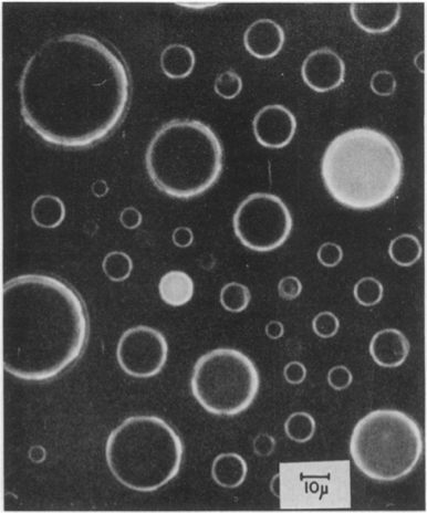
The heterogeneity in the drops is obvious. Drops showed quantized activities proportional to the number of enzyme copies in the droplet.
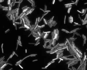
We can also see heterogeneity if we look at gene expression in bacterial cells. In the image below, we see an image of E. coli cells expressing yellow fluorescent protein (YFP) under control of the LacI promoter. The variation in fluorescent intensity, and therefore gene expression level, is apparent.
Types of noise
To quantitatively define noise, it helps to perform a thought experiment. Say we have many exactly identical cells. At some point in the future, as gene expression, responses to the environment (which we assume is the same for each cell), etc. proceed, the cells will no longer be identical due to stochasticity in all of these processes involving small numbers of molecules. Consider one gene product of interest in these cells (such as YFP in the image above). We can define the total noise, \(\eta_\mathrm{tot}\), as the coefficient of variation of the copy numbers of the gene product. The coefficient of variation is the standard deviation of the copy number divided by the mean copy number, or
\begin{align} \eta_\mathrm{tot}^2 = \frac{\left\langle n^2\right\rangle - \left\langle n\right\rangle ^2}{\left\langle n\right\rangle ^2}, \end{align}
where \(n\) is the copy number. If the standard deviation is comparable to the mean, as we would expect in the case of large copy numbers, we have low noise, but if it is large compared to the mean, we have high noise.
Continuing with the thought experiment, we might have fluctuations in environmental conditions that might change the expression level of the gene of interest, either directly, or indirectly through expression of other genes in any given cell. We might also have fluctuations in gene expression due to the inherent stochasticity present in cellular processes, such as in those involved in the Central Dogma. This leads us to categorize the noise according to intrinsic and extrinsic noise.
Intrinsic noise: Transcription and translation can occur at different times and rates in otherwise identical systems. This results in fluctuations in \(n(t)\). The fluctuations in the copy number of the protein of interest are due to fluctuations that affect only the gene of interest. Operationally, intrinsic noise causes the failure of identical genes in identical environments to correlate. This fundamentally limits the precision of regulation.
Extrinsic noise: Other molecular species, such as RNA polymerase, ribosomes, and chemical species in the cell’s environment, vary over time and affect the gene of interest. The fluctuations in the copy number of the protein of interest are due to fluctuations that affect all genes in a cell.
Experimentally determining intrinsic and extrinsic noise
Measurement of noise, both intrinsic and extrinsic, is necessary. It is really hard to know a priori how intrinsically noisy gene expression will be without measuring it. The problem is that just measuring cell-cell variation does not separate intrinsic noise in the process of gene expression from extrinsic cell-cell variation in key cellular components, such as ribosomes, polymerases, etc. Moreover, even if there were no extrinsic noise at all, intrinsic noise can still depend on the relative transcription, translation, and degradation rates, or other factors we are not aware of. Thus, it is critical to actually measure it and see how it behaves.
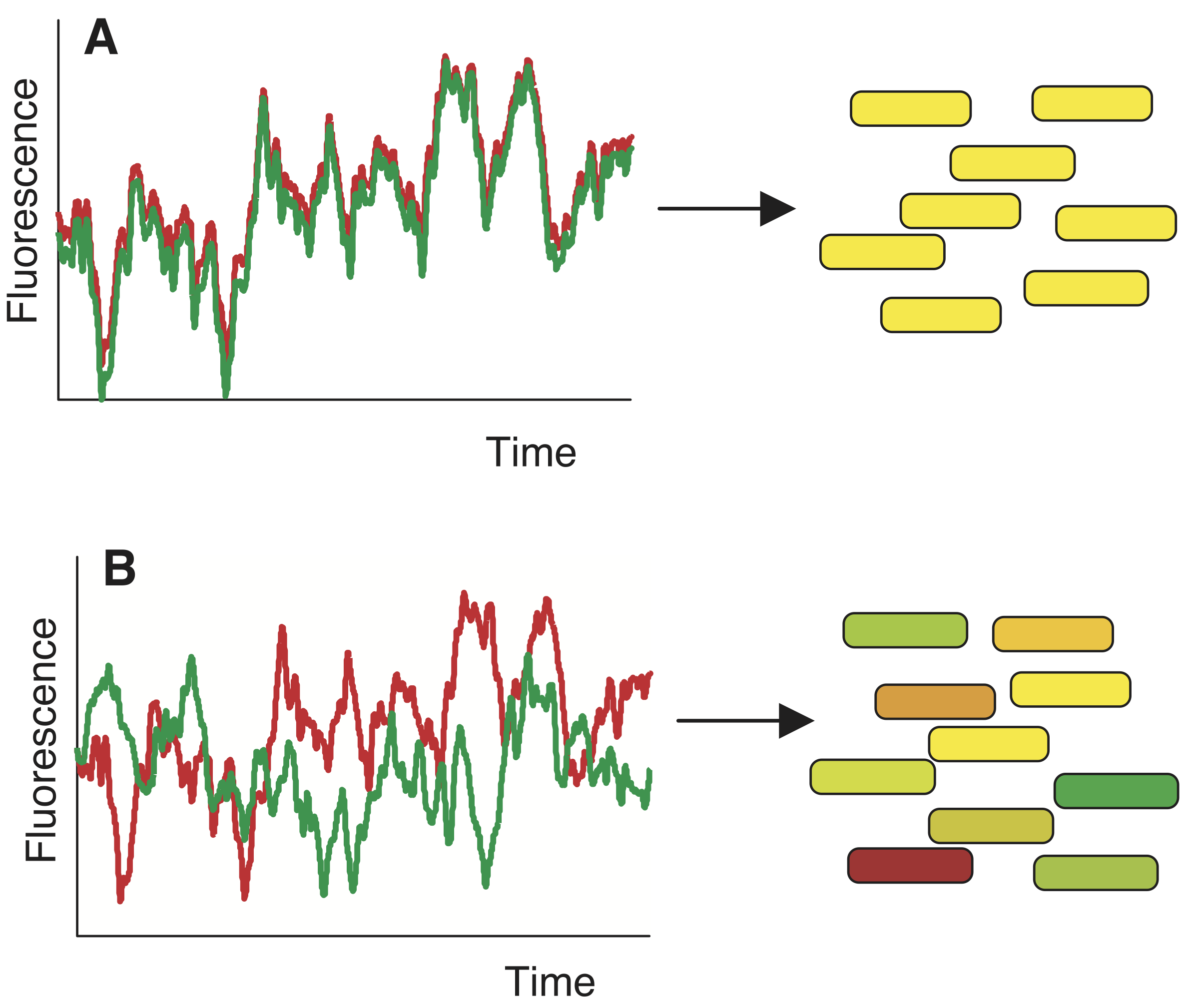
Delineating intrinsic and extrinsic noise is difficult, if not impossible, by measuring expression of a single gene in a cell. To construct an experiment to study this, we can conduct another thought experiment. Say we put two perfectly, molecularly identical cells in the exact same environment and see if they behave similarly. Unfortunately, we cannot do this, because we cannot prepare two perfectly identical cells. However, we can put two (nearly) identical genes in the same cell. This is conceptually related, and allows us to think of these two genes as two independent stochastic samples of the same underlying process. If everything behaved deterministically and was only influenced by extrinsic noise, we would expect strongly correlated variation in both genes, as in panel A of the image below. If, however, expression is non-deterministic then variation will be uncorrelated, as in panel B, below.
To perform this experiment Elowitz and coworkers (Science, 2002) developed a system in which identical promoters were used to express fluorescent proteins of different color, cyan fluorescent protein (CFP) and YFP. The promoters were repressed by the LacI protein. They could tune the repression by changing concentration of IPTG, since IPTG inhibits LacI’s ability to act as a repressor.
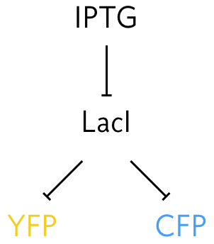
They were also careful to integrate the promoters into the genome at loci that were equidistant from the origin of replication so that the copy number of each on the chromosome remains the the same as the genome is replicated. They then could measure the expression level for identical promoters under identical conditions, since the promoters are in the same cell. A typical result is shown in the images below.
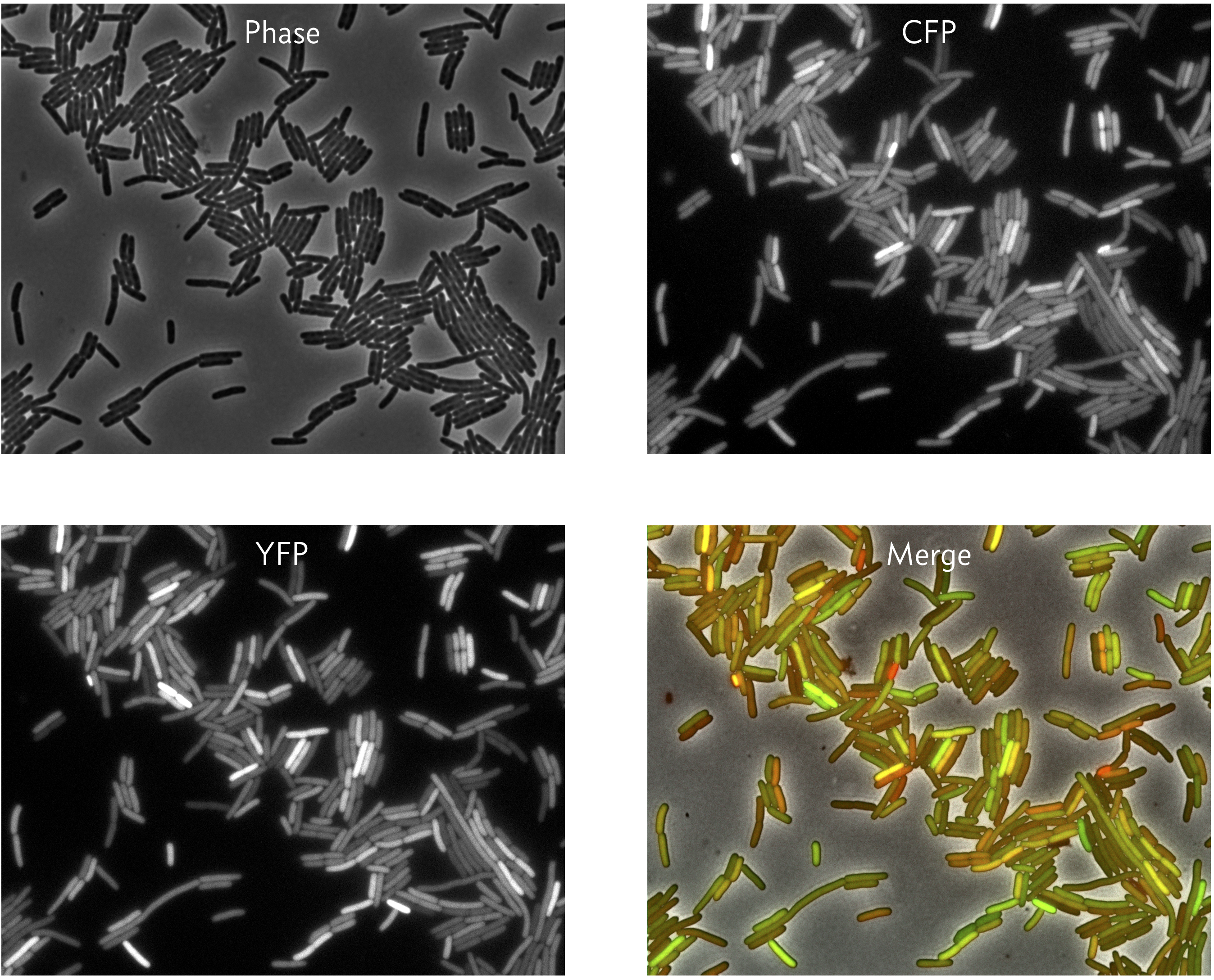
We can see that in some cells, both the CFP and YFP levels are high (yellow in the merge), but in other cases, they CFP and YFP levels differ (green or red in the merge).
The rest of this chapter addresses how we can separate intrinsic from extrinsic noise from images like these.
Segmentation and scaling of fluorescence
First, the images must be segmented, which means that each pixel in the image needs to be labeled with a unique number corresponding to which bacterium (or background) it belongs. The phase contrast image is used for this purpose because it is generally bad practice to use the signal you are trying to measure in segmentation. Next, the intensities of the pixels in each channel (CFP and YFP) for each bacterium are summed to give a total intensity. The integrated CFP intensity for cell \(i\) is
\begin{align} c_i = c_0 n_{c,i}, \end{align}
where \(n_{c,i}\) is the copy number of CFP in cell \(i\). The constant \(c_0\) is determined by the fluorescent yield of YFP, microscope settings, etc. Similarly, the integrated YFP intensity for cell \(i\) is
\begin{align} y_i = y_0 n_{y,i}. \end{align}
It is in general very difficult to measure \(c_0\) or \(y_0\). While we could have more sophisticated statistical models to try to ascertain them, we will instead scale the YFP intensity such that
\begin{align} \langle y \rangle = \langle c \rangle. \end{align}
The assumption in doing so is that the mean copy number of YFP and CFP are equal. This is an important assumption, which hopefully holds because of the careful construction of the promoters on the chromosome, and is one we will rely on going forward.
In practice, if \(\{c_i, y_i\}\) is the set of \(N\) cellular CFP and YFP integrated intensities we measured and
\begin{align} \bar{c} = \frac{1}{N}\sum_{i=1}^N c_i, \\[1em] \bar{y} = \frac{1}{N}\sum_{i=1}^N y_i \end{align}
are the arithmetic mean of the CFP and YFP intensities, we adjust
\begin{align} c_i \leftarrow c_i / \bar{c},\\[1em] y_i \leftarrow y_i / \bar{y}, \end{align}
which enforces that the means are equal (and both arbitrarily equal to one). With the redefinition, the prefactors connecting the fluorescent intensity to copy number are equal, or \(c_0 = y_0\).
Plug-in estimates for intrinsic, extrinsic, and total noise
As our first approach to estimating the intrinsic and extrinsic noise from our data set \(\{c_i, y_i\}\), let us assume that we do not know the probability distribution describing \(\{c_i, y_i\}\). Since we do not know the distribution, we will resort to making plug-in estimates of the moments of the distribution to estimate quantities such as \(\langle n^2 \rangle\). Remember that going forward, we assume that the data have already been properly scaled to have the same mean.
To compute the total noise, we need to compute the variance in gene expression. Since both CFP and YFP are on identical promoters, we can group them together as a single species in this calculation. The plug-in estimate for the total variance is then
\begin{align} V_\mathrm{tot} = \frac{1}{2N}\sum_{i=1}^N\left[\left(c_i - \bar{c}\right)^2 + \left(y_i - \bar{y}\right)^2\right] = \frac{1}{2}\left(\overline{c^2} - \bar{c}^2 + \overline{y^2} - \bar{y}^2\right). \end{align}
The factor in the denominator is \(2N\) because we have two fluorescent species in each cell.
The intrinsic noise comes from within-cell variation. This is quantified by the difference in fluorescence between the CFP and YFP fluorescence in each cell. This variation is quantified by the mean-square difference,
\begin{align} V_\mathrm{int} = \frac{1}{2N}\sum_{i=1}^N\left(c_i - y_i\right)^2 = \frac{1}{2}\left(\overline{c^2} + \overline{y^2}\right) - \overline{cy}. \end{align}
Note that we again divide by two because both the CFP and YFP expression are subjected to the same intrinsic noise. Since \(V_\mathrm{int}\) accounts for the intrinsic variance, we define the remainder of the variance to be due to extrinsic noise,
\begin{align} V_\mathrm{ext} = V_\mathrm{tot} - V_\mathrm{int} = \overline{cy} - \frac{1}{2}\left(\bar{c}^2 + \bar{y}^2\right) = \overline{cy} - \bar{c}\bar{y}, \end{align}
where in the last equality we have used the fact that \(\bar{c} = \bar{y}\). We recognize that the extrinsic noise is given by the plug-in estimate for the covariance. We can now write expressions for the plug-in estimates for the noise by dividing these variances by the square of the mean expression, \(\bar{c}\bar{y}\) (again, because \(\bar{c} = \bar{y}\)).
\begin{align} &\eta_\mathrm{tot}^2 = \frac{V_\mathrm{tot}}{\bar{c}\bar{y}} = \frac{1}{2\bar{c}\bar{y}}\left(\overline{c^2} - \bar{c}^2 + \overline{y^2} - \bar{y}^2\right),\\[1em] &\eta_\mathrm{int}^2 = \frac{V_\mathrm{int}}{\bar{c}\bar{y}} = \frac{1}{2\bar{c}\bar{y}}\left(\overline{c^2} + \overline{y^2}\right) - \overline{cy}\\[1em] &\eta_\mathrm{ext}^2 = \frac{V_\mathrm{ext}}{\bar{c}\bar{y}} = \frac{\overline{cy} - \bar{c}\bar{y}}{\bar{c}\bar{y}}. \end{align}
Computing the intrinsic and extrinsic noise from experimental data
As an example, let us compute the intrinsic and extrinsic noise from experimental data. We will consider two data sets from the Elowitz, et al. paper, both of which are contained in this CSV file. One set of measurements is for the M22 strain, which has the CFP/YFP under control of LacI setup in E. coli we have previously described. The other set of measurements is for the D22 strain, which has a deletion of the recA gene, which is responsible for rescuing stalled replication forks.
Let’s plot the two data sets and compare.
[2]:
# Read in the data set
df = pd.read_csv(os.path.join(data_path, "elowitz_et_al_2002_fig_3a.csv"))

# Extract measurements into Numpy arrays
m22_cfp = df.loc[
    (df["strain"] == "m22") & (df["fluorophore"] == "cfp"), "intensity"
].values
m22_yfp = df.loc[
    (df["strain"] == "m22") & (df["fluorophore"] == "yfp"), "intensity"
].values
d22_cfp = df.loc[
    (df["strain"] == "d22") & (df["fluorophore"] == "cfp"), "intensity"
].values
d22_yfp = df.loc[
    (df["strain"] == "d22") & (df["fluorophore"] == "yfp"), "intensity"
].values

# Scale the measurements by their means
m22_cfp /= m22_cfp.mean()
m22_yfp /= m22_yfp.mean()
d22_cfp /= d22_cfp.mean()
d22_yfp /= d22_yfp.mean()

# Generate plot
p = bokeh.plotting.figure(
    frame_width=250, frame_height=250, x_axis_label="CFP", y_axis_label="YFP"
)
p.circle(m22_cfp, m22_yfp, alpha=0.3, legend_label="M22")
p.circle(d22_cfp, d22_yfp, color="orange", alpha=0.3, legend_label="D22")
p.legend.location = "bottom_right"
p.legend.click_policy = "hide"
p.legend.background_fill_alpha = 0.7

bokeh.io.show(p)
The apparent positive covariance is indicative of the presence of extrinsic noise. We will now proceed to compute plug-in estimates for the intrinsic, extrinsic, and total noise.
[3]:
def plugin_noise(c, y):
    """Plug-in estimates for noise"""
    Vtot = np.var(np.concatenate((c, y)), ddof=0)
    Vext = np.cov(c, y, ddof=0)[0, 1]
    Vint = Vtot - Vext

    return np.sqrt(np.array([Vint, Vext, Vtot]) / c.mean() / y.mean())


# Compute plug-in estimates
m22_noise = plugin_noise(m22_cfp, m22_yfp)
d22_noise = plugin_noise(d22_cfp, d22_yfp)

# Print the result
print(
    """
M22
---
intrinsic: {0:.4f}
extrincic: {1:.4f}
total:     {2:.4f}

D22
---
intrinsic: {3:.4f}
extrincic: {4:.4f}
total:     {5:.4f}
""".format(
        *m22_noise, *d22_noise
    )
)
M22
---
intrinsic: 0.0554
extrincic: 0.0540
total:     0.0774

D22
---
intrinsic: 0.0814
extrincic: 0.0809
total:     0.1147
We can compute confidence intervals on these values using pairs bootstrap.
[4]:
# Function to draw a pairs bootstrap replicate
def draw_bs_rep(c, y):
    bs_inds = np.random.choice(np.arange(len(c)), len(c))
    bs_c, bs_y = c[bs_inds], y[bs_inds]
    return plugin_noise(bs_c, bs_y)


# Generate bootstrap replicates
n_reps = 100000
m22_reps = np.array([draw_bs_rep(m22_cfp, m22_yfp) for _ in range(n_reps)])
d22_reps = np.array([draw_bs_rep(d22_cfp, d22_yfp) for _ in range(n_reps)])

# Compute 95% confidence interval
m22_confint = np.percentile(m22_reps, [2.5, 97.5], axis=0)
d22_confint = np.percentile(d22_reps, [2.5, 97.5], axis=0)
Now that we have the confidence intervals, we can plot our estimates for the noise with the 95% confidence interval.
[5]:
# Organize results for convenient plotting
noises = ["intrinsic", "extrinsic", "total"]
strains = ["M22", "D22"]
noise = [m22_noise, d22_noise]
confint = [m22_confint.T, d22_confint.T]
data = [
    ((s, n), confint[i][j, 0], confint[i][j, 1], noise[i][j])
    for i, s in enumerate(strains)
    for j, n in enumerate(noises)
]
df_noise = pd.DataFrame(
    columns=["strain_noise", "2.5", "97.5", "plugin"], data=data
)

# Build data source and factor range for plot
y_range = bokeh.models.FactorRange(*df_noise["strain_noise"][::-1])
source = bokeh.models.ColumnDataSource(df_noise)

# Build the plot
p = bokeh.plotting.figure(y_range=y_range, height=200, x_axis_label="noise")
p.circle(x="plugin", y="strain_noise", source=source)
for _, row in df_noise.iterrows():
    p.line([row["2.5"], row["97.5"]], [row["strain_noise"]] * 2, line_width=2)

bokeh.io.show(p)
It is also interesting to plot our bootstrap samples to see how the intrinsic and extrinsic noise are correlated.
[6]:
p = bokeh.plotting.figure(
    frame_width=250,
    frame_height=250,
    x_axis_label="intrinsic noise",
    y_axis_label="extrinsic noise",
)
p.circle(m22_reps[::40, 0], m22_reps[::40, 1], alpha=0.1, legend_label="M22")
p.circle(
    d22_reps[::40, 0],
    d22_reps[::40, 1],
    alpha=0.1,
    color="orange",
    legend_label="D22",
)
p.legend.location = "bottom_right"

bokeh.io.show(p)
There is slight anticorrelation between intrinsic and extrinsic noise.
Interpreting the results
Apparently, for genes regulated by LacI in E. coli, the intrinsic and extrinsic noise are of similar magnitude. The D22 string is inherently noisier, with the noise being about 50% higher than the M22 strain. Importantly, this suggests that the difference in noise is genetically determined. That the role of recA in rescuing stalled replication forks and the fact that it is missing in the D22 strain suggests that the increased noise, both intrinsic and extrinsic, is due to transient copy number differences between different parts of the chromosome.
Generative Bayesian modeling of noise
In the above analysis, we assumed we knew nothing about underlying probability distribution generating the data. This means we are not modeling the source of the noise, but are rather defining what we mean by intrinsic and extrinsic noise based on moments of the unknown distribution, which we then estimate with plug-in estimates. We now take an alternative approach, where we propose a generative model for the data. The parameters of this model then define what we mean by intrinsic and extrinsic noise. We use Bayes’s theorem to connect the experimental measurements to the noise, given the model.
One of the beauties of generative modeling is that all assumptions are now, by necessity, explicit. We will again make the same assumptions we did when deriving the plug-in estimates, stating them more clearly here.
The mean fluorescence is equal for the CFP and YFP channels.
The copy number is linearly related to the measured fluorescence.
There is no background fluorescence.
All noise is inherent to the genetic machinery of the bacteria; there is no measurement error.
The fluorescent intensity of each cell is independent of all other cells and also identically distributed (i.i.d).
Although under these assumptions the measured fluorescence should take on discrete values, we nonetheless model the fluorescence values as continuous.
The assumption of no measurement error was not apparent in the nonparametric analysis. We assumed we knew nothing about the distribution that produced the experimental measurements, but we then chose to interpret the plug-in estimates as they relate to genetic noise, ignoring measurement noise.
To build our parametric model, we must first build a probability distribution for the likelihood of the data. This is the probability distribution describing observation of our data set. Because of the i.i.d. assumption, we can consider a single cell, \(i\). Then, our modeling means we specify the joint probability density function \(P(c_i, y_i\mid \theta_i)\) where \(\theta_i\) is a set of parameters that condition the observations.
While not necessary at this point, for concreteness, we will model this distribution as Normal, such that
\begin{align} c_i \sim \mathrm{Norm}(\mu_i, \sigma_i),\\[1em] y_i \sim \mathrm{Norm}(\mu_i, \sigma_i), \end{align}
where \(\theta_i = \{\mu_i, \sigma_i\}\). Here, \(\sigma_i\) explicitly characterizes within cell variability of expression of the gene of interest; it gives the intrinsic noise. If we assume that every cell experiences the same intrinsic noise, then \(\sigma_i = \sigma\;\forall i\), and
\begin{align} c_i \sim \mathrm{Norm}(\mu_i, \sigma),\\[1em] y_i \sim \mathrm{Norm}(\mu_i, \sigma), \end{align}
or
\begin{align} P(c_i, y_i \mid \mu_i, \sigma) = \frac{1}{2\pi\sigma^2}\exp\left[-\frac{(c_i - \mu_i)^2 + (y_i - \mu_i)^2}{2\sigma^2}\right]. \end{align}
The extrinsic noise affects the expression level of all genes; that is it affects variability in \(\mu_i\). We can model the \(\mu_i\)’s as varying from a set value \(\mu\) with standard deviation \(\sigma_\mu\) according to a Gaussian distribution,
\begin{align} \mu_i \sim \mathrm{Norm}(\mu, \sigma_\mu), \end{align}
or
\begin{align} P(\mu_i\mid \mu, \sigma_\mu) = \frac{1}{\sqrt{2\pi\sigma_\mu^2}}\,\exp\left[-\frac{(\mu_i-\mu)^2}{2\sigma_\mu^2}\right]. \end{align}
The parameter \(\sigma_\mu\) is related to the extrinsic noise. We can therefore define the intrinsic and extrinsic noise as
\begin{align} &\eta_\mathrm{int} = \frac{\sigma}{\mu},\\[1em] &\eta_\mathrm{ext} = \frac{\sigma_\mu}{\mu}. \end{align}
To complete the generative model, we need to specify prior distributions on the parameters \(\mu\), \(\sigma\), and \(\sigma_\mu\); that is, we need to specify \(P(\mu, \sigma, \sigma_\mu)\). We will leave that unspecified for now, and will proceed to write down Bayes’s theorem for this hierarchical model.
\begin{align} P(\{\mu_i\}, \mu, \sigma, \sigma_\mu\mid \{c_i, y_i\}) \propto \left(\prod_{i=1}^N P(c_i, y_i \mid \mu_i, \sigma) P(\mu_i\mid \mu, \sigma_\mu)\right) P(\mu, \sigma, \sigma_\mu). \end{align}
Performance of full Bayesian inference on this model involves some sophisticated techniques involving Markov chain Monte Carlo, which we will not cover here. Most important for this chapter is that we can build a generative model and directly and intuitively interpret its parameters.
Computing environment
[7]:
%load_ext watermark
%watermark -v -p numpy,pandas,bokeh,jupyterlab
Python implementation: CPython
Python version       : 3.8.8
IPython version      : 7.22.0

numpy     : 1.20.1
pandas    : 1.2.4
bokeh     : 2.3.1
jupyterlab: 3.0.14