8. Robustness in biological circuits
Design principles
Exact adaptation, such as that displayed by the chemotaxis circuit in E. coli, can be achieved through integral feedback.
Techniques
Michaelis-Menten kinetics to model enzyme dynamics.
Concepts
Robustness.
Exact adaptation.
[1]:
# Colab setup ------------------
import os, sys, subprocess
if "google.colab" in sys.modules:
    cmd = "pip install --upgrade colorcet biocircuits watermark"
    process = subprocess.Popen(cmd.split(), stdout=subprocess.PIPE, stderr=subprocess.PIPE)
    stdout, stderr = process.communicate()
# ------------------------------

import numpy as np
import scipy.integrate

import biocircuits.apps

import bokeh.io
import bokeh.models
import bokeh.plotting

import colorcet

# Set to True to have access to fully interactive plots
fully_interactive_plots = False
notebook_url = "localhost:8888"

bokeh.io.output_notebook()
The principle of robustness (demonstrated with dosage compensation)
You have likely heard the word robustness used in biological contexts, possibly even in the context of biological circuits. You may have a feeling for what is meant when we talk about robustness, but it is important to have a precise definition. We will begin with the following operational definition.
A property of a biological circuit is robust if it is nearly independent of some of the biochemical parameters that vary unavoidably from cell to cell or system to system.
Let us think about how we could apply this definition to some circuits we have already considered.
Robustness and the I1-FFL dosage compensation circuit
We have studied dosage compensation by an I1-FFL architechture. As a reminder, the unregulated and regulated circuit responding to copy number \(C\) are shown below.

We derived that the steady state concentration of Y for copy number \(C\) is
\begin{align} y_\mathrm{ss} = \frac{C^n}{1 + \beta^n C^n}, \end{align}
where \(\beta = \beta_y/k\gamma\) is the ratio of the unregulated steady state level of Y at unit copy number and \(\gamma\) is the decay rate of Y. From this expression, we see that if \(n = 1\) and \(\beta \gg 1\) (or if \(C\) is very large), \(y_\mathrm{ss} \approx 1/\beta\). We can then construct a statement of robustness:
For the I1-FFL dosage compensation circuit sketched above, the steady state concentration of Y is robust to variations in copy number \(C\) in the regime where \(\beta C \gg 1\). In general, since \(C \ge 1\), \(\beta \gg 1\) is sufficient to ensure robustness.
How to make statements about robustness
The structure of the above statement about a robustness property I1-FFL circuit has the following form (where X, Y, and Z do not refer to genes in the above circuit, but are generic properties).
Property X of the system is robustto variations in Yin operating regime Z.
To fully specify what we mean by robustness in a given context, we must specify
The property (X);
To what variations the property is robust (Y);
In what regime Z the robustness holds.
Any other statement about robustness is incomplete. Never say, “The I1-FFL dosage compensation circuit is robust.” That means nothing.
Anti-robustness: Fine-tuned
A system or property of a system that is not robust is said to be fine-tuned. A fine-tuned property of a circuit requires precise adjustment of biochemical parameters to maintain its function. Just like robustness, we need to define X, Y, and Z as above: what property we are talking about, what parameter variations will destroy its function, and in what regime these variations have that effect. We can say the following for the I1-FFL dosage compensation circuit.
The I1-FFL dosage compensation is not robust to copy number fluctuations if the Hill coefficient \(n\) is anything other than unity.
Robustness in the C1-FFL circuit function
As a second example of robustness, let us consider the design principle we found in a previous chapter: The C1-FFL with AND logic displays an on-delay. We saw that this property of the C1-FFL holds even when the Hill coefficient for the regulation is unity. We might also ask if the delay is robust to variations in the Hill activation constants.
As a reminder, the dimensionless dynamical equations for the concentrations of Y and Z from a stimulus X are
\begin{align} \frac{\mathrm{d}y}{\mathrm{d}t} &= \beta\,\frac{(\kappa x)^{n_{xy}}}{1 + (\kappa x)^{n_{xy}}} - y, \\[1em] \gamma^{-1}\frac{\mathrm{d}z}{\mathrm{d}t} &= \frac{x^{n_{xz}} y^{n_{yz}}}{(1 + x^{n_{xz}})\,(1+ y^{n_{yz}})} - z. \end{align}
To investigate the effect of the Hill activation constants, we need only to vary the dimensionless parameter \(\kappa\), which is the ratio of the Hill activation constant for activation of Z by X to the Hill activation constant for activation of Z by Y; \(\kappa = k_{xz}/k_{yz}\). Note that the dimensionless \(\beta\) was defined by \(\beta \leftarrow \beta/\gamma_y k_{xy}\), so neither of the Hill activation constants in \(\kappa\) appear in other parameters. However, the dimensionless concentration of Y includes \(k_{yz}\). Nonetheless, neither Hill activation constant appears in the nondimensionalziation of Z.
We can again use the functions we previously developed that are in the FFL app in the biocircuits package. We will use the same parameter values as in the last lesson, but we will vary \(\kappa\). We can then plot the time it takes the level of Z to reach half its steady state value versus \(\kappa\) to investigate how the robust the delay time is to variations in \(\kappa\). For reasons that will become clear in a moment, we will also plot the maximal Z-concentration.
[2]:
# Parameter values
beta = 5
gamma = 1
n_xy, n_yz = 3, 3
n_xz = 5
logic = "and"
x_args = (0, 10, 1)
t_step_down = 11
x_0 = 10
t = np.linspace(0, 10, 2000)

# Initial condition
yz0 = np.array([0, 0])

# Solve for delays
y_delay = []
y_max = []
z_delay = []
z_max = []
kappa = np.logspace(-2, 2, 200)
for kap in kappa:
    y, z = biocircuits.apps.solve_ffl(
        beta, gamma, kap, n_xy, n_xz, n_yz, "c1-ffl", logic, t, t_step_down, x_0
    ).transpose()

    # Store the delays and max's
    y_max.append(y.max())
    y_delay.append(t[np.nonzero(y > 0.5 * y.max())[0][0]])
    z_max.append(z.max())
    z_delay.append(t[np.nonzero(z > 0.5 * z.max())[0][0]])

# Plot the delays
p1 = bokeh.plotting.figure(
    width=300,
    height=200,
    x_axis_label="κ",
    y_axis_label="time to half max",
    x_axis_type="log",
)
p1.circle(kappa, y_delay, color="orange", legend_label="y")
p1.circle(kappa, z_delay, legend_label="z")

# Plot the max levels
p2 = bokeh.plotting.figure(
    width=300,
    height=200,
    x_axis_label="κ",
    y_axis_label="steady state level",
    x_axis_type="log",
    y_axis_type="log",
)
p2.circle(kappa, y_max, color="orange")
p2.circle(kappa, z_max)

bokeh.io.show(bokeh.layouts.row(p1, bokeh.models.Spacer(width=50), p2))
Apparently for small \(\kappa\), the delay time is longer. However, for small \(\kappa\), we also see that the response of \(z\) very rapidly drops to zero. With \(\kappa = 0.1\), the response is seven orders of magnitude smaller than for \(\kappa = 1\). This falls off far more rapidly than the steady state level of \(y\). So, we really do not have any response of Z below \(\kappa \approx 0.5\). As \(\kappa\) gets large, the delay time is nonzero and invariant to \(\kappa\), as is the steady state. In this regime of large \(\kappa\), regardless the magnitude of \(\kappa\), it takes Z about 50% longer to reach its steady state than Y. So, we can make a robustness statement:
The on-delay of the C1-FFL and steady state Z levels are robust to changes in the ratio of the Hill activation constants, \(\kappa\) when \(\kappa\) is large.
We could do a more careful survey of parameter values, varying strength of expression \(\beta\), the hight of the input step \(x_0\), the ratio of the decay constants \(\gamma\), and the Hill coefficients to get quantitative bounds on the range of \(\kappa\) values that preserve the on-delay and steady state levels.
Why it is good to be robust
For a living organism robustness is important to ensure that components work reliably in the face of the inevitable variations it will face. We will talk more about stochastic noise in future lessons, but it is also important to note that circuits may be robust to parameter variations that occur due to random mutation over generations.
For a bioengineer, robustness is a key concept in identifying effective circuit architectures. If the properties we are trying to design in a circuit are robust, there is more “slop” in the design.
A case study in robustness: E. coli chemostaxis
To demonstrate how we assess robustness of biological circuits, we will now perform a case study on the Che system of E. coli, largely based on Chapter 7 of Alon’s book.
When flagellated, E. coli can swim toward attractants and away from repellents. Ideally, they swim up (in the case of attractants) the gradient in attractant concentration. This means that the bacteria perform a differentiation calculation, measuring the change in attractant concentrations as they move through space as opposed to the absolute level of attractant concentration.
To understand how this is accomplished, we must first understand how E. coli swim. Their flagellar motors spin in an anticlockwise direction when they are being propelled forward in a so-called “run.” Occasionally, a few of the motors switch to a clockwise rotation, which causes the bacterium to stall and spin in a so-called “tumble.” When the motors switch to spinning anticlockwise, the bacterium runs again in a new, random direction.
If a bacterium is swimming up a gradient of attractant, its switching frequency decreases and it continues up the gradient. If however, there is no gradient, but perhaps a more uniform concentration of attractant, the switching frequency should return back to the level it was before detecting the gradient. This leads to a statement about robustness: The steady state tumbling frequency of the Che system is robust to variations in total attractant concentration. It turns out that the operating regime over five orders of magnitude of total attractant concentration!
The switching frequency is controlled by the Che system, shown in the image below.
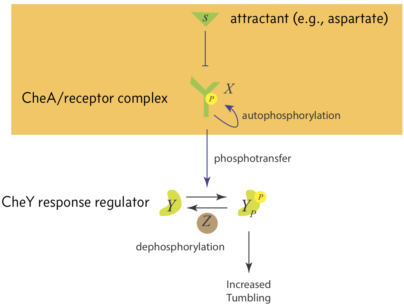
The CheA receptor complex, which we shall call X, is autophosporylated. Attractant serves to inhibit autophosphorylation of CheA, thereby inhibiting phosphorylation of CheY. This then leads to a decrease in tumbling rate.
We will focus on the mechanism of CheA phosphorylation in response to attractants, shown in the orange box in the above figure. To enable the steady state tumbling frequency to be invariant to total attractant concentration, we always want the level of phosphorylated CheA to return to the same steady state regardless of the attractant concentration. This feature of a circuit, wherein it returns to the same steady state after an adjustment of its input (in this case, the attractant concentration) is called exact adaptation.
We will be focusing on the exact adaptation aspects of this circuit. For a beautiful description of how swimming bacteria compute gradients for foraging, you should read the classic paper by Berg and Purcell.
The CheA circuit
Zooming in now on the CheA circuit (the orange box in the figure above), the CheA receptor can exist in methylated and demethylated states. The methylation state is controlled by the methylating enzyme CheR and the demethylating enzyme CheB. Furthermore, the CheA receptor can have an active conformation and an inactive conformation. The presence of attractant pushes the CheA receptor toward the inactive state. A schematic for a possible mechanism for this is shown in the image below.
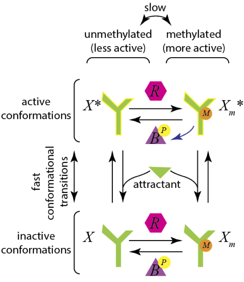
The combination of being in the active and methylated state results in a much more active receptor, so we will be most interested in the concentration of \(X_m^*\). We will model all of the enzyme kinetics using Michaelis-Menten kinetics, and we pause for a moment to work out the mathematical expressions.
Michaelis-Menten kinetics
At the heart of a Michaelis-Menten description of enzyme kinetics is the following set of chemical reactions between the enzyme E and substrate S to give product P.
\begin{align} E + S \stackrel{k}{\rightleftharpoons} ES \stackrel{v}\rightarrow P + E. \end{align}
The idea is that the enzyme reversibly binds the substrate with binding rate constant \(k_+\) and unbinding rate constant \(k_-\). When bound, the enzyme can serve to convert the substrate to product with rate constant \(v\) Applying mass action kinetics, we can write the dynamics as a system of ordinary differential equations.
\begin{align} \frac{\mathrm{d}c_e}{\mathrm{d}t} &= -\frac{\mathrm{d}c_{es}}{\mathrm{d}t} = -k_+c_e c_s + (k_- + v)c_{es},\\[1em] \frac{\mathrm{d}c_s}{\mathrm{d}t} &= -k_+c_sc_e + k_-c_{es},\\[1em] \frac{\mathrm{d}c_p}{\mathrm{d}t} &= v c_{es}, \end{align}
where \(c_i\) denotes the concentration of species i. Note that
\begin{align} \frac{\mathrm{d}c_e}{\mathrm{d}t} + \frac{\mathrm{d}c_{es}}{\mathrm{d}t} = 0, \end{align}
which is a statement of conservation of enzyme. This means that we need to specify a total enzyme amount to fully specify the problem. We define this to be \(c_e^0\) such that \(c_e^0 = c_e + c_{es}\). With this conservation law, we can write the ODEs as
\begin{align} \frac{\mathrm{d}c_{es}}{\mathrm{d}t} &= k_+(c_e^0-c_{es}) c_s - (k_- + v)c_{es},\\[1em] \frac{\mathrm{d}c_s}{\mathrm{d}t} &= -k_+(c_e^0-c_{es})c_s + k_-c_{es},\\[1em] \frac{\mathrm{d}c_p}{\mathrm{d}t} &= v c_{es}. \end{align}
These equations describe the full dynamics of the enzyme catalyzed system. To simplify the analysis, we often make the quasi-steady state approximation that the bound substrate intermediate ES does not see appreciable change in its concentration on the time scale of the production of the product P. That is,
\begin{align} \frac{\mathrm{d}c_{es}}{\mathrm{d}t} = k_+(c_e^0-c_{es}) c_s - (k_- + v)c_{es} \approx 0. \end{align}
This enables us to solve for the quasi-steady state fraction of enzyme that is bound to substrate.
\begin{align} \frac{c_{es}}{c_e^0} \approx \frac{c_s/K}{1 + c_s/K}, \end{align}
where we have defined the Michaelis constant
\begin{align} K = \frac{v + k_-}{k_+}. \end{align}
It has dimension of concentration and is analogous to a dissociation constant in that it is the ratio of the total rate constant for dissociation of the enzyme from the catalyst to that of binding the enzyme to the catalyst.
Substitution of this expression gives
\begin{align} \frac{\mathrm{d}c_p}{\mathrm{d}t} \approx v\,c_e^0\, \frac{c_s/K}{1 + c_s/K}. \end{align}
By conservation of mass, if \(\mathrm{d}c_{es}/\mathrm{d}t \approx 0\), then
\begin{align} \frac{\mathrm{d}c_s}{\mathrm{d}t} \approx -\frac{\mathrm{d}c_p}{\mathrm{d}t} \approx -vc_e^0\, \frac{c_s/K}{1 + c_s/K}. \end{align}
Testing the accuracy of the quasi-steady state approximation
To test the accuracy of the pseudo-steady state approximation, it helps, as usual, to nondimensionalize the variables. We perform the nondimensionalization as follows.
\begin{align} t &\leftarrow k_- t,\\[1em] c_{es} &\leftarrow \frac{c_{es}}{c_e^0},\\[1em] c_s &\leftarrow \frac{c_s}{K},\\[1em] c_p &\leftarrow \frac{c_p}{K}. \end{align}
The dimensionless dynamical equations are then
\begin{align} \kappa\, \frac{\mathrm{d}c_{es}}{\mathrm{d}t} &= (1-c_{es}) c_s - c_{es},\\[1em] \zeta^{-1} \frac{\mathrm{d}c_s}{\mathrm{d}t} &= -(1-c_{es})c_s + \kappa \,c_{es},\\[1em] \frac{\mathrm{d}c_p}{\mathrm{d}t} &= \zeta(1-\kappa)c_{es}. \end{align}
We have defined two dimensionless parameters. First, we have
\begin{align} \kappa = \frac{k_-}{v + k_-}. \end{align}
which is the probability that a given enzyme-substrate complex will end up dissociating back to separated enzyme and substrate as opposed being converted to product. Second, noting that the dissociation constant for enzyme-substrate is \(K_d = k_-/k_+\), we have
\begin{align} \zeta = \frac{k_+ c_e^0}{k_-} = \frac{c_e^0}{K_d}. \end{align}
This is how much enzyme we have in units of \(K_d\).
It is apparent in looking at the dimensionless equations that the quasi-steady state approximation is valid when \(\zeta\) is small (we do not have too much enzyme). To investigate this, we can make plots and compare the solution to the full dynamical equations and those using the quasi-steady state approximation. In the plot below, we show the approximate dynamics of the substrate and the product as fainter colored lines.
You must be running an active Jupyter notebook to fully interact with the below plot.
[3]:
def michaelis_menton_rhs(c, t, kappa, zeta):
    ces, cs, cp = c
    return np.array(
        [
            ((1 - ces) * cs - ces) / kappa,
            zeta * (-(1 - ces) * cs + kappa * ces),
            zeta * (1 - kappa) * ces,
        ]
    )


def approx_michaelis_menton_rhs(c, t, kappa, zeta):
    cs, cp = c
    deriv = zeta * (1 - kappa) * cs / (1 + cs)
    return np.array([-deriv, deriv])


kappa_slider = bokeh.models.Slider(
    title="κ", start=0.01, end=1, value=0.5, step=0.01, width=200
)
zeta_slider = bokeh.models.Slider(
    title="ζ",
    start=-2,
    end=2,
    value=0,
    step=0.05,
    width=200,
    format=bokeh.models.FuncTickFormatter(code="return Math.pow(10, tick).toFixed(2)"),
)


def solve_mm(kappa, zeta):
    # Initial condition
    c0 = np.array([0.01, 10, 0.01])

    # Time points
    t = np.linspace(0, 100, 400)

    # Solve the full system
    c = scipy.integrate.odeint(michaelis_menton_rhs, c0, t, args=(kappa, zeta))
    ces, cs, cp = c.transpose()

    # Solve the approximate system
    c_approx = scipy.integrate.odeint(
        approx_michaelis_menton_rhs, c0[1:], t, args=(kappa, zeta)
    )
    cs_approx, cp_approx = c_approx.transpose()

    return t, ces, cs, cp, cs_approx, cp_approx


# Get solution for initial glyphs
t, ces, cs, cp, cs_approx, cp_approx = solve_mm(
    kappa_slider.value, 10 ** zeta_slider.value
)

# Set up ColumnDataSource for plot
cds = bokeh.models.ColumnDataSource(
    dict(t=t, ces=ces, cs=cs, cp=cp, cs_approx=cs_approx, cp_approx=cp_approx)
)

# Make the plot
p = bokeh.plotting.figure(
    plot_width=500,
    plot_height=250,
    x_axis_label="t",
    y_axis_label="dimensionless concentration",
    y_axis_type="linear",
    x_range=[0, 100],
)

colors = colorcet.b_glasbey_category10

# Populate glyphs
p.line(
    source=cds, x="t", y="ces", line_width=2, color=colors[0], legend_label="ES",
)
p.line(
    source=cds, x="t", y="cs", line_width=2, color=colors[1], legend_label="S",
)
p.line(
    source=cds, x="t", y="cp", line_width=2, color=colors[2], legend_label="P",
)
p.line(
    source=cds, x="t", y="cs_approx", line_width=4, color=colors[1], alpha=0.3,
)
p.line(
    source=cds, x="t", y="cp_approx", line_width=4, color=colors[2], alpha=0.3,
)

p.legend.location = "center_right"


if fully_interactive_plots:

    def callback(attr, old, new):
        """Callback to update data for new plot"""
        t, ces, cs, cp, cs_approx, cp_approx = solve_mm(
            kappa_slider.value, 10 ** zeta_slider.value
        )
        cds.data = dict(
            t=t, ces=ces, cs=cs, cp=cp, cs_approx=cs_approx, cp_approx=cp_approx
        )

    # Link sliders
    kappa_slider.on_change("value", callback)
    zeta_slider.on_change("value", callback)

    layout = bokeh.layouts.column(
        kappa_slider,
        bokeh.models.Spacer(height=10),
        zeta_slider,
        bokeh.models.Spacer(height=10),
        p,
    )

    def app(doc):
        doc.add_root(layout)

    bokeh.io.show(app, notebook_url=notebook_url)
else:
    kappa_slider.disabled = True
    zeta_slider.disabled = True
    slider_layout = bokeh.layouts.row(
        bokeh.layouts.column(kappa_slider, bokeh.models.Spacer(height=10), zeta_slider),
        bokeh.layouts.Spacer(width=30),
        bokeh.layouts.column(
            bokeh.layouts.Spacer(height=20),
            bokeh.models.Div(
                text="""
<p>Sliders are inactive. To get active sliders, re-run notebook with
<font style="font-family:monospace;">fully_interactive_plots = True</font>
in the first code cell.</p>
        """,
                width=250,
            ),
        ),
    )
    layout = bokeh.layouts.column(slider_layout, p,)

    bokeh.io.show(layout)
In manipulating the sliders, we see that, indeed, if \(\zeta\) is small (that is we do not have too much enzyme), then the concentration of ES quickly goes to a steady level while the concentration of product grows. The approximate solution to the Michaelis-Menten dynamics, at least for production of product, very closely follows that obtained for the full dynamics.
Approximate dynamics of the Che signaling system
Because of the more verbose names of the species in the Che system (e.g., “\(X_m^*\)” instead of “S”), we will denote concentrations of respective species with lower case letter, e.g. \(x_m^*\).
We will assume that the quasi-steady state approximation holds for all enzyme-catalyzed reactions. We assume further that CheR operates at saturation. This means that there is so much substrate (in this case unmethlyated CheA receptor complex) such that the rate of methylation by CheR is directly proportional to the CheR concentration, or
\begin{align} \frac{r/K_R}{1+r/K_R} \approx 1. \end{align}
When this is the case, it is said that CheR operates at saturation.
We can write an ODE for the rate of change of total methylated CheA. At steady state, this derivative vanishes.
\begin{align} \frac{\mathrm{d}(x^*_m + x_m)}{\mathrm{d}t} = \frac{\mathrm{d}x_m^\mathrm{tot}}{\mathrm{d}t} = 2v_R r - v_B b\left(\frac{x_m^*/K_m}{1 + x_m^*/K_m} + \frac{x_m/\kappa_m}{1 + x_m/\kappa_m}\right) = 0, \end{align}
where \(K_m\) and \(\kappa_m\) are Michaelis constants for demethylation by CheB. This equation is readily solved for \(x_m^*\).
\begin{align} x_m^* = K_m\,\frac{2 v_R r - v_B b\,\frac{x_m/\kappa_m}{1 + x_m/\kappa_m}}{v_B b - 2v_R r + v_B b\,\frac{x_m/\kappa_m}{1 + x_m/\kappa_m}} \end{align}
Note that as \(x_m\) grows, the numerator decreases, while the denominator increases. So, for increasing \(x_m\), \(x_m^*\) decreases. Because the amount of \(x_m\) is dependent on the amount of attractant present (more attractant means the equilibrium shifts toward the inactive conformations, \(x\) and \(x_m\)), the concentration of active CheA receptor complex is dependent on the attractant concentration in this model.
Fine-tuned exact adaptation
We an imagine a scenario where we could get exact adaptation in tumbling frequency from this circuit. If the attractant affects the phosphotransfer and the CheY response, we can write
\begin{align} \text{tumbling frequency} \equiv A = a(L)\,x_m^*, \end{align}
where \(L\) is the concentration of attractant ligand and \(a(L)\) is some function. Before the attractant was present, we have a tumbling frequency of \(A_0 = a_0 x_{m,0}^*\), and after we have \(A_1 = a_1 x_{m,1}^*\), where \(a_0 = a(L_0)\) and \(a_1 = a(L_1)\). Note that addition of attractant also shifts the balance between methylated and unmethylated CheA receptor complex, so \(x_m\) is affected. We define
\begin{align} \theta = 2v_r r - v_b b\,\frac{x_m/\kappa_m}{1 + x_m/\kappa_m}. \end{align}
Then, the concentration of active methylated CheA complex is
\begin{align} x_m^* = K_m\,\frac{\theta}{v_B b - \theta}. \end{align}
With this expression, we can write down the two tumbling frequencies.
\begin{align} A_0 = a_0 x_{m,0}* = a_0 K_m \,\frac{\theta_0}{v_B b - \theta_0}, \\[1em] A_1 = a_1 x_{m,1}* = a_1 K_m \,\frac{\theta_1}{v_B b - \theta_1}. \end{align}
For exact adaptation, for this particular concentration of attractant, \(A_0 = A_1\), or
\begin{align} \frac{a_1}{a_0} = \frac{\theta_1(v_B b - \theta_0)}{\theta_0(v_B b - \theta_1)}. \end{align}
The problem is that this ratio must hold for any \(a_0\) and \(a_1\) within an operating regime if exact adaptation is to be robust. This results in a delicate balancing act, since \(\theta\) changes with varying attractant concentration. This is an example of fine-tuning. Exact adaptation is only possible by precisely setting parameters for a given pair of attractant concentrations, and the exact adaptation is lost if those attractant concentrations change at all.
Robust exact adaptation
Let us now assume a different architecture of the Che circuit. We will assume that CheB only demethylates active receptors, rendering them inactive. The circuit diagram in this case is
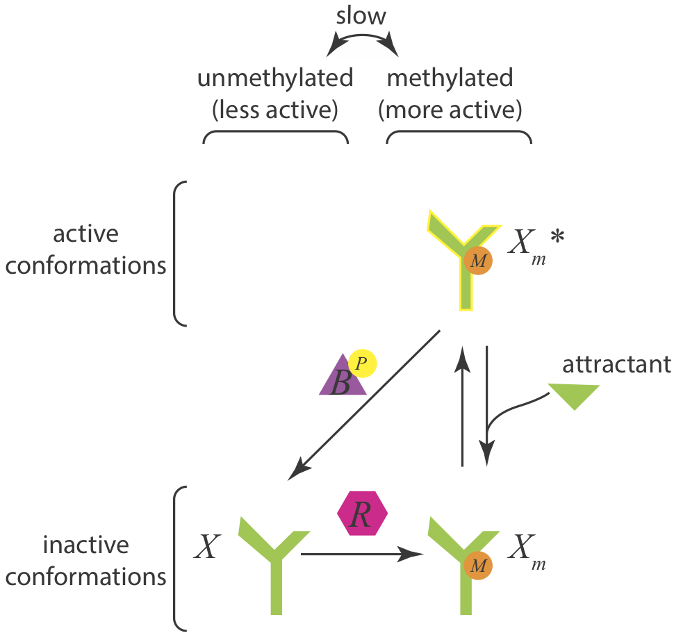
Taking the same approach as before, we can again write down the dynamics for the total amount of methylated CheA complex. We will again assume that CheR is operating at saturation.
\begin{align} \frac{\mathrm{d}(x_m +x_m^*)}{\mathrm{d}t} = v_R r - v_B b\,\frac{x_m^*/K_m}{1+x_m^*/K_m}. \end{align}
At steady state, the time derivative vanishes, and we have
\begin{align} x_m^* = K_m\,\frac{v_R r}{v_B b - v_R r}. \end{align}
This is independent of \(x_m\), and is dependent only on the parameters and concentrations pertaining to the CheB and CheR enzymes. If we have the simplest model where \(a(L) = \text{constant}\), then exact adaptation is achieved over all attractant concentrations. Furthermore, exact adaptation is robust to variations in parameter values (like CheR concentration, \(v_B\), etc.), provided the Michaelis-Menten kinetics are valid and CheR operates at saturation.
Note, however, that the steady state tumbling frequency is not robust to changes in parameter values. The exact adaptation is robust to changes in parameter values, but the level of the steady state has explicit dependence on them and is therefore not robust to fluctuations in parameter values.
A more complex model for chemotaxis
In the model for chemotaxis that we have considered, there are only two methylation states of the receptor, either unmethylated or methylated. In a more general model, we could consider multiple methylation states of the receptor. That is, it could be unmethylated, once methylated, twice methylated, …, m-times methylated. Such a system was analyzed computationally by Barkai and Leibler (1997).
Because the model for generic number of methylation states is not tractable analytically as the one we have considered, Barkai and Leibler instead did a computational exploration of the parameter space. They began with a set of \(n\) parameters \(k_1^0\), \(k_2^0\), …, \(k_n^0\). They randomly varied these parameters to get a new set of parameters \(k_1\), \(k_2\), …, \(k_n\). They defined the total parameter variation \(K\) according to
\begin{align} \ln K = \sum_{i=1}^n \left|\ln\,\frac{k_i}{k_i^0}\right|. \end{align}
For this new set of parameters, they solved the system of ODEs numerically from a steady state in response to an abrupt step up in ligand. If the probability of being in an active state for the original set of parameters is \(A_0\) and for the perturbed parameters is A, then the precision of adaptation, \(P\), is defined as \(P = A_0 / A\).
The results from thousands of such perturbations and calculations of the precision of adaptation is shown below. This image was taken from the Barkai and Liebler paper (which unfortunately has the Nature Publishing Group watermark on it).
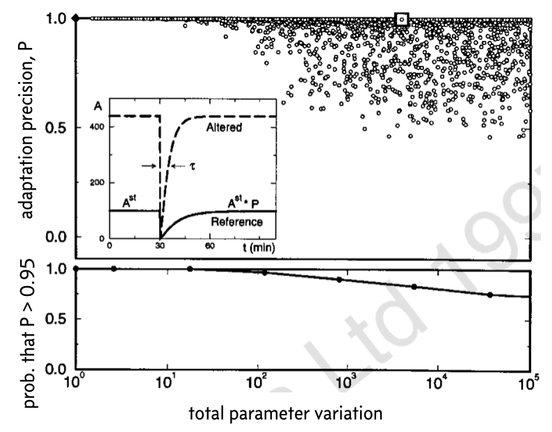
In the top plot, the diamond represented the original set of parameters. In the inset, the response for the original set of parameters is shown (solid line) along with an example response, corresponding to the white box.
To make clear the overlapping points in the top plot, the bottom plot shows the fraction of parameter sets for which the precision of adaptation \(P < 0.95\) for various values of the total parameter variation \(K\). These plots demonstrate that even over large degrees of parameter variation, up to a total of four or five orders of magnitude, the system can still achieve rather exact adaptation.
Conversely, Barkai and Leibler found that the time to steady state is not robust to parameter variations.
Exact adaptation in the Che system is robust to CheR levels, as shown experimentally
In a follow-up experimental paper (Alon, et al., 2000), the authors varied CheR expression levels by putting CheR under control of the lac promoter and varying the concentrations of IPTG. They used microscopy to observe the tumbling frequency of cells. They spiked in a saturating amount of attractant and observed the tumbling frequency over time. The results from their experiment are shown below, reproduced from the paper.
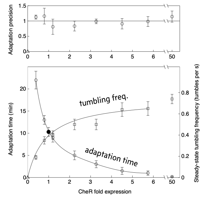
Commensurate with the model predictions, the precision of adaptation is robust to varying levels of CheR over about two orders of magnitude. They also found that the time it took to reach a steady state tumbling frequency and the steady state frequency itself were not robust to varying levels of CheR.
Integral feedback
The chemotaxis system we have studied in this lesson achieves exact adaptation robustly via a mechanism called integral feedback control, as first noticed by Yi and coworkers. The key features of integral feedback control are:
The steady state is independent of external perturbation.
The system tends toward steady state as time tends toward infinity; i.e., it is asymptotically stable.
The time integral of error is fed back into the system.
A block diagram for integral control is shown below. The desired output is \(y_0\) and the actual output is \(y\), so the error is \(e = y_0 - y\). This error is integrated over time, multiplied by a gain \(k\), and then added to the a perturbation \(u\). In the context of the chemotaxis system, the perturbation is the change in attractant concentration.
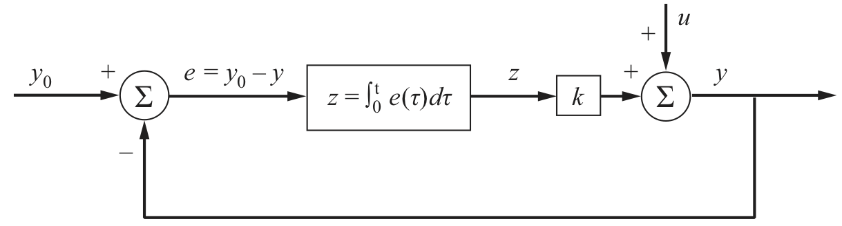
Image from Del Vecchio and Murray, Biomolecular Feedback Systems, Princeton University Press, 2015.
If we write ODEs for this diagram, we have that
\begin{align} \frac{\mathrm{d}z}{\mathrm{d}t} = e(t) = y_0 - y, \end{align}
with \(y = kz + u\), giving
\begin{align} \frac{\mathrm{d}z}{\mathrm{d}t} = e(t) = y_0 - kz - u. \end{align}
The steady state is then \(y = y_0\), which is asymptotically stable if the gain \(k\) is positive and the perturbation is constant (such as a change in attractant concentration). In the present case, the term \(kz\) represents the linearized balance between methylated and unmethylated CheA receptor complex. Importantly, the integral feedback ensures that the steady state is independent of the perturbation \(u\).
You can read more about integral feedback in section 3.2 of Del Vecchio and Murray’s book and in this very nice primer on control theory in synthetic biology by Swaminathan, Hsiao, and Murray.
Computing environment
[4]:
%load_ext watermark
%watermark -v -p numpy,scipy,bokeh,biocircuits,jupyterlab
Python implementation: CPython
Python version       : 3.8.8
IPython version      : 7.22.0

numpy      : 1.20.1
scipy      : 1.6.2
bokeh      : 2.3.1
biocircuits: 0.1.3
jupyterlab : 3.0.14