17. Time-based regulation in cells
Design principle
Time-based regulation enables coordinated regulation of target genes
Frequency Modulated Pulsing can implement time-based regulation
Concepts
In time-based regulation, as opposed to concentration-based regulation, inputs control the fraction of time a regulator is active, rather than the concentration of the active species.
Techniques
Autocorrelation and cross-correlation analysis
[1]:
import numpy as np
import scipy.stats as st

import bokeh.io
import bokeh.plotting

bokeh.io.output_notebook()
Biological circuits can be strikingly dynamic, even in constant conditions
Even in a constant environment, biological circuits exhibit surprisingly dynamic behaviors. One can observe proteins activating and deactivating in repetitive pulses or or periodic oscillations across a wide range of timescales. Indeed, we have already seen how just a few genes can produce robust oscillations. In many cases, dynamics are coherent, involving simultaneous activation and deactivation of many molecules of a given species.
Today we will ask what functional benefits dynamics can provide for a signaling system compared to non-dynamic alternatives. We will see that dynamics allows cells to control targets “in time” rather than in concentration, and that this time-based regulation can allow coordination of diverse target genes within the cell.
Electrical systems also use dynamics
Electrical circuit design utilizes dynamics for numerous operations. One of the simplest, and most familiar, examples is a classic “dimmer” switch. Dimmers control light intensity by rapidly chopping the voltage on and off, varying the fraction of time that the light is on.
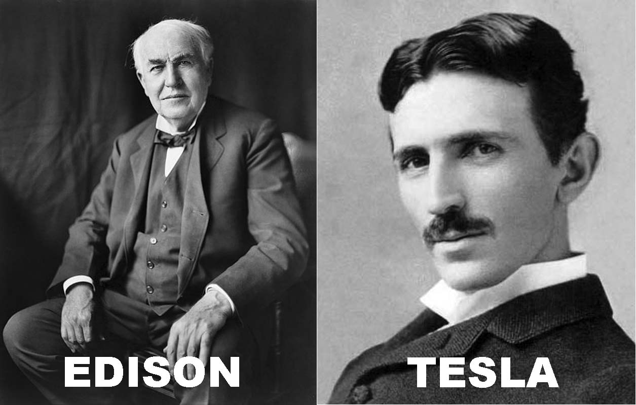
Our electrical devices are a mix of AC (alternating current) and DC (direct current) designs. The complementary benefits of the two paradigms are sometimes associated with the legendary conflict between Edison and Tesla, who advocated competing visions for DC and AC power distribution, respectively. The AC model prevailed for power distribution, while DC power is better for many digital electronic systems, such as laptop computers.
AM and FM represent distinct signal encoding paradigms
In communications, signals can be encoded either in the amplitude or frequency of oscillations. Car stereos usually offer both Amplitude Modulation (AM) and Frequency Modulation (FM) radio bands. In either case, one can tune the radio to a particular frequency or channel. AM radios encode signals in the amplitude of that frequency, while FM encodes signals via small shifts in frequency. The code below shows two very simple ways of encoding the same information:
[2]:
t = np.linspace(0, 25, 1001)

# Frequency of carrier signal
f = 1

# Carrier signal
yc = np.sin(2 * np.pi * f * t)

# Modulation signal
m = np.sin(2 * np.pi * 0.1 * f * t)

# Phase multiplier
pm = 4

# Amplitude modulation
AM = m * yc

# Modulate phase to give frequency modulated signal
FM = np.sin(2 * np.pi * (f * t + pm * m))

# Collect signals for convenience
signals = dict(carrier=yc, signal=m, AM=AM, FM=FM)

# Set up plots
colors = bokeh.palettes.d3["Category10"][4]
plots = [
    bokeh.plotting.figure(
        height=150, width=400, x_axis_label="time" if key == "FM" else None, title=key
    )
    for key in signals
]

# Link axes
for p in plots[1:]:
    p.x_range = plots[0].x_range
    p.y_range = plots[0].y_range

# Populate glyphs
for i, (key, sig) in enumerate(signals.items()):
    plots[i].line(t, sig, line_width=2, color=colors[i])

bokeh.io.show(bokeh.layouts.gridplot(plots, ncols=1))
Transcription factors can be regulated in concentration or in time
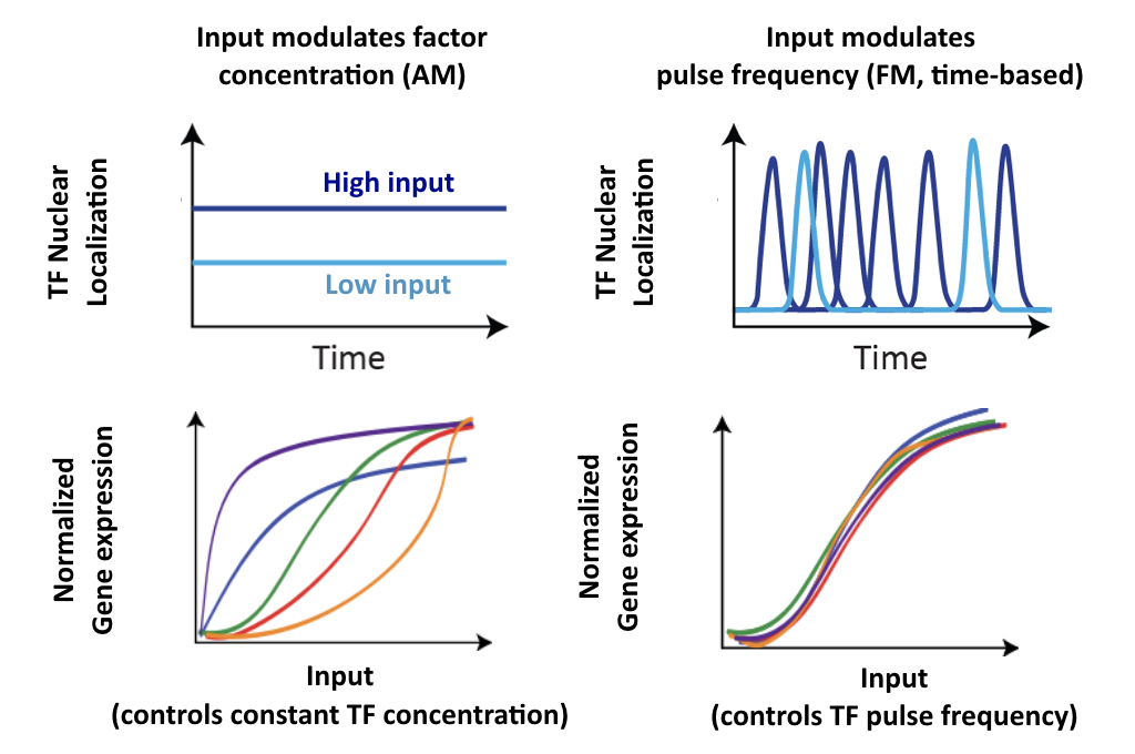
Cellular signaling systems can similarly encode inputs in qualitatively different ways:
In an AM-like concentration-based encoding system, the input signals controls the concentration of an effector inside the cell. This is how we typically assume most systems work.
In a time-based regulation system, the input signal can modulate dynamic aspects of a signal, such as its oscillatory period, or, as we will discuss today, the fraction of time that the regulator is active.
These two modes are illustrated schematically here:
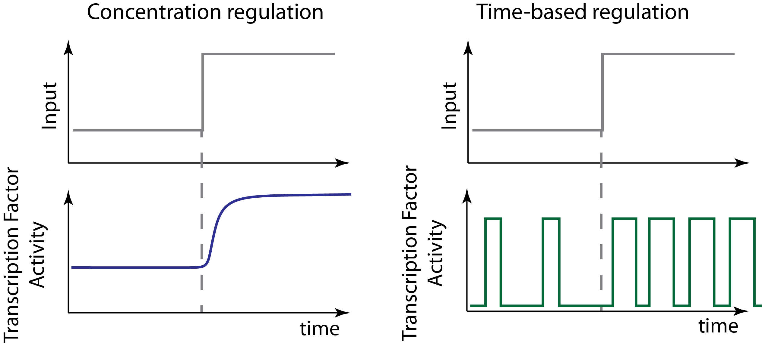
Note that in this schematic example of time-based regulation, we allow the input to modulate both the frequency and duration of pulses to change the fraction of time that the factor is active. But there are many ways to implement time-based regulation. And any given system may mix both of these or other types of regulation at the same time.
Dynamic pulsing is ubiquitous
A large, and ever-growing, list of regulatory systems and pathways exhibit repetitive pulses of activity in constant conditions. In bacteria, sigma factors activate in pulses. In yeast, key transcription factors mediating stress response or glucose regulation, such as Msn2, Crz1, and Mig1, exhibit repetitive pulses of nuclear localization. In mammalian cells, core signaling pathways including NF-AT, NF-\(\kappa\)B, Erk, p53, and others all exhibit different types of pulsing even when cells are in constant conditions. Examples of these systems are summarized in this figure, which shows pulses from a broad variety of different cell types:
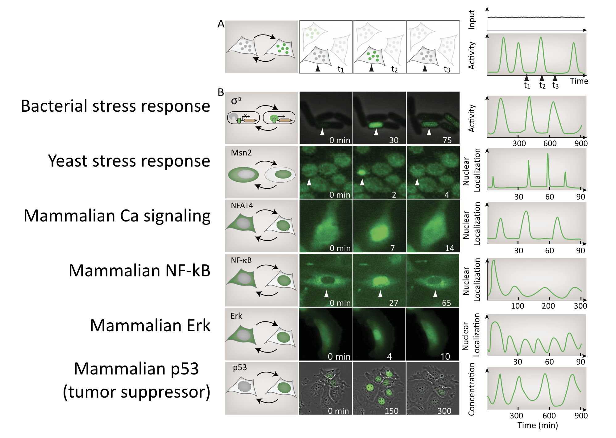
Image from Levine, Lin, and Elowitz (Science, 2013)
Detecting pulsing is not easy, since it requires making movies of specific regulators in individual cells. For this reason, this list is almost certainly an underestimate of the number and diversity of pulsatile factors.
In fact, a systematic movie-based survey of all yeast proteins detected pulsatile dynamics in at least some conditions for about 10% of transcription factors. This work took advantage of a convenient property of many transcription factors. They localize to the nucleus when they are active, and to the cytoplasm when they are inactive.
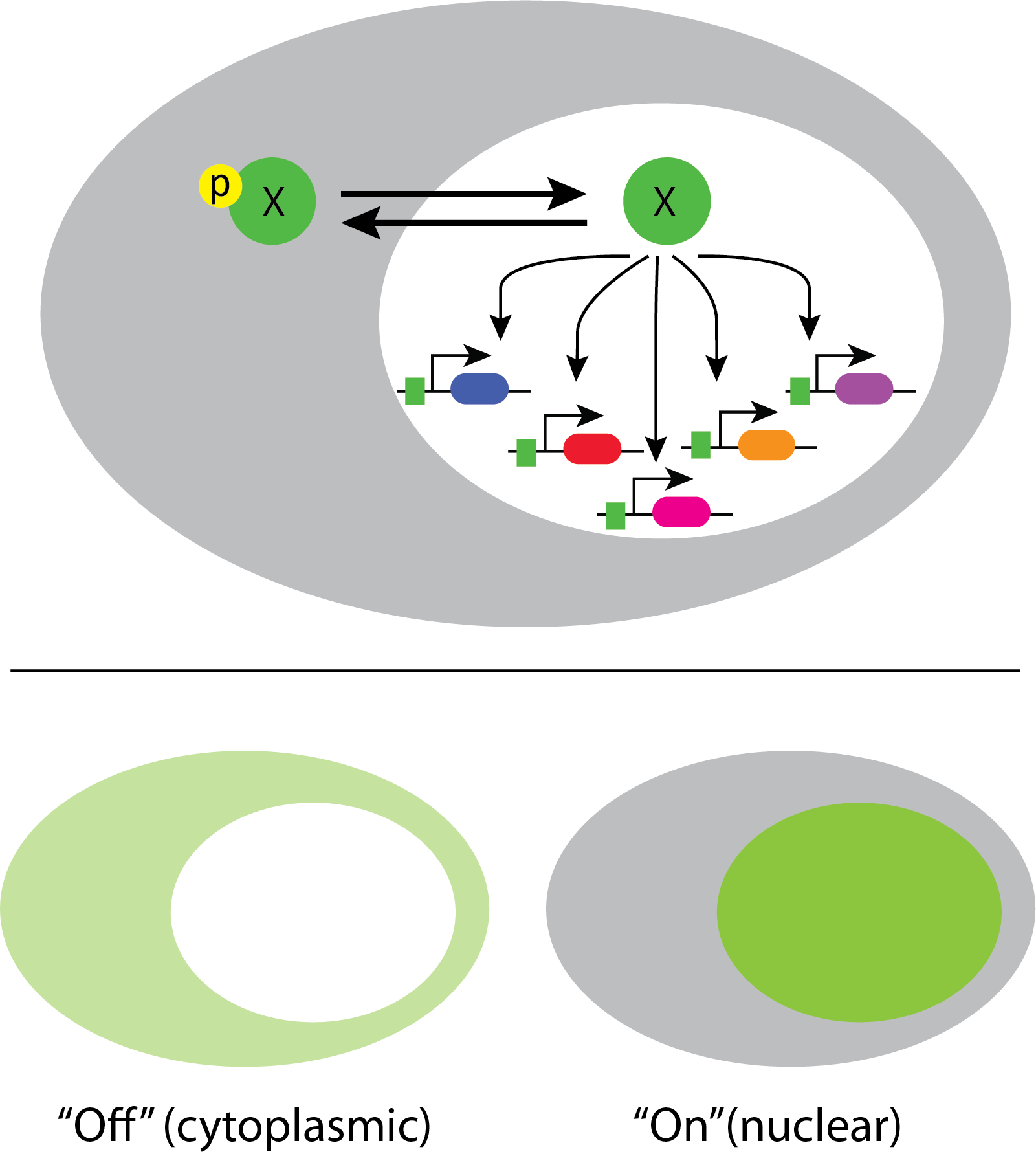
This enables one to infer total transcription factor activity from the degree of nuclear localization, as shown in these movies:
Movie from C. Dalal et al (Current Biology, 2014).
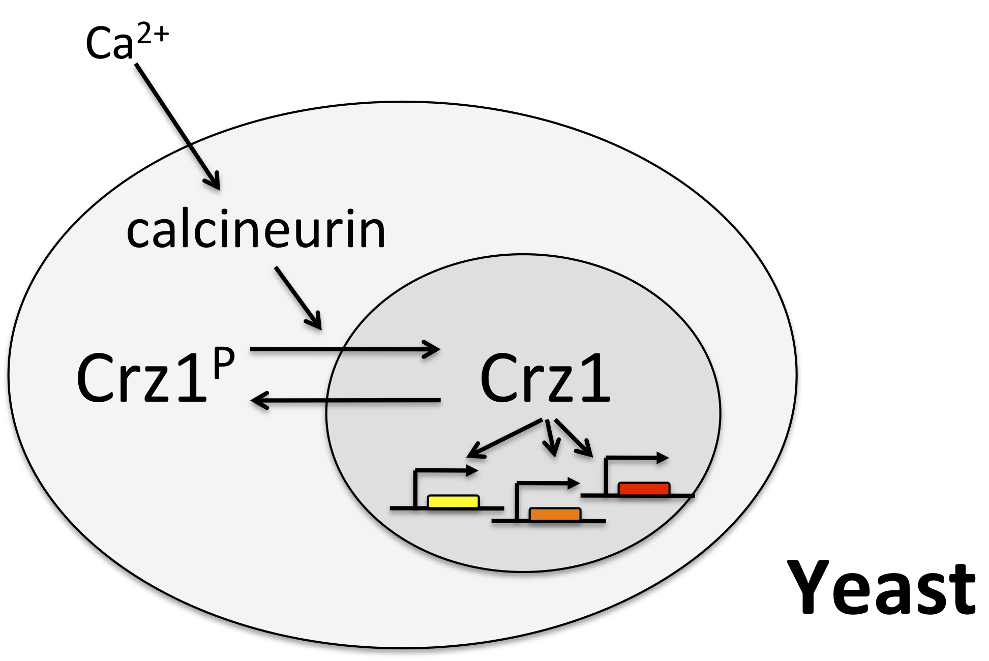
Crz1 mediates the response to calcium through nuclear localization
One of the best examples of this mode of control is the yeast transcription factor Crz1, whose name stands for calcineurin-responsive zinc finger 1, and is pronounced “crazy one.”
In this system, calcium activates the phosphatase calcineurin, which dephosphorylates Crz1. The desporphorylated form localizes to the nucleus, where it can activae a large regulon of target genes. Crz1 is functionaly analogous to the NF-AT transcription factors that play critical roles in the immune system, among many other texts. (See Stathopoulos, et al. (Genes Dev., 1997, *Genes Dev., 1999; and Matheos et al. (Genes Dev., 1997).)
Crz1 pulses
In the late 2000s, Crz1 earned its name. Here at Caltech, Long Cai and Chiraj Dalal, working in Elowitz lab, were making movies of individual yeast cells expressing Crz1 fused to a fluorescent protein. After addition of calcium to the media, they were struck by the mesmerizing and unexpected “twinkling” of individual cells. These twinkles represented events in which many Crz1 molecules simultaneously transited to the nucleus, concentrating their fluorescent signal. They lasted for a couple of minutes and then ended as the Crz1 proteins returned to the cytoplasm. These cycles of coherent, repetitive pulses of nuclear localization continued for hours. The following movie shows a typical example.
Pulses appear stochastic and (sometimes) repetitive
To get a better idea of what is going on in this system, one can plot traces of Crz1 nuclear localization over time. For example, here are traces from two neighboring cells:
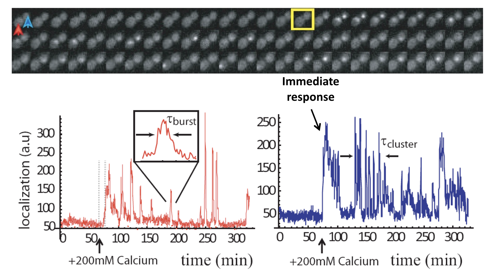
Analysis of Crz1 pulse dynamics in two cells, from L. Cai et al. (Nature, 2008)
These traces show a number of interesting features:
Nuclear localization occurs in brief pulses (sometimes called spikes or bursts), typically lasting just a couple of minutes. These pulses occur only after calcium is added to the media.
Pulses are unsynchronized between different cells, indicating they are generated in a cell-autonomous way. In fact, pulsing is uncorrelated even between mother-daughter cell pairs.
In many, but not all, cells, one sees an immediate response to sudden addition of calcium. This occurs in the blue trace, above.
One also can frequently observe extended episodes of elevated pulsing rate, termed pulse “trains” or “clusters.”
These features could only be discerned because we looked at individual cells over time. Averaging over many of these traces reveals a very different population average behavior, in which there is an initial response, evidently due to synchronized response to calcium addition, followed by partial adaptation to an (apparently) constant level. Of course, this seemingly steady behavior conceals the wild pulsing going on in each individual cell.
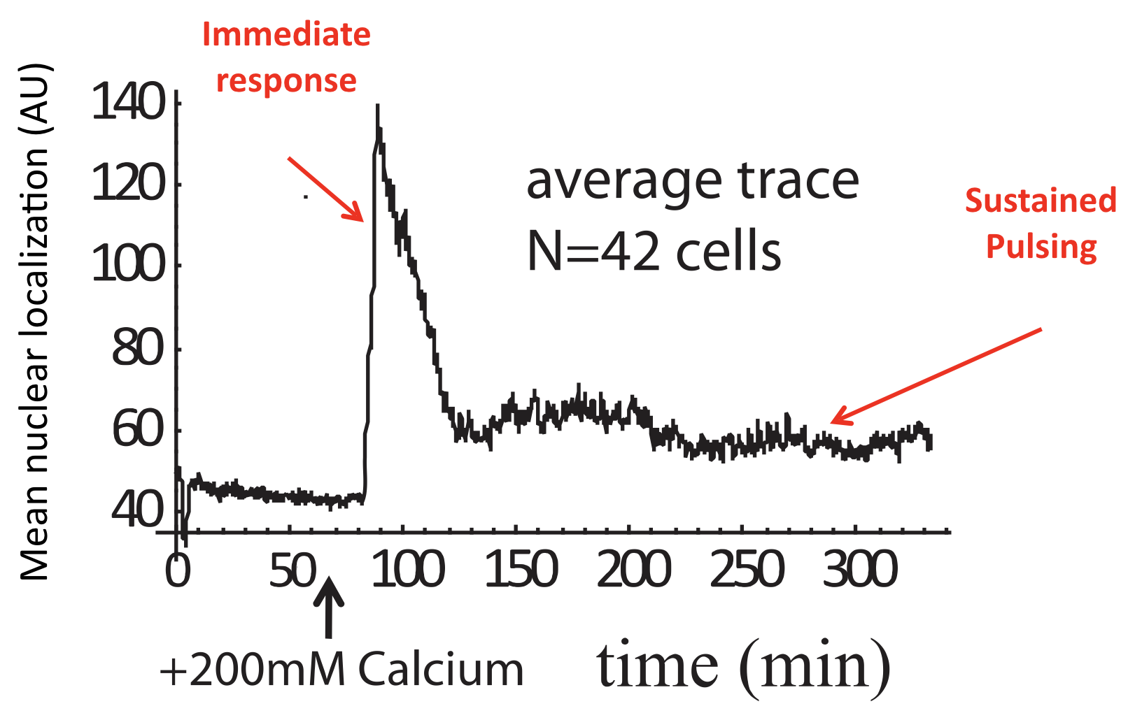
Average of Crz1 pulse dynamics in 42 cells, from L. Cai et al. (Nature, 2008).
Dynamic correlation analysis allows extraction of key features of stochastic dynamics
These observations present us with a frequently encountered challenge: How to condense a huge number of distinct, individual behaviors, each occurring in a different cell, into a small number of comprehensible parameters.
One of the most versatile tools is correlation analysis.
Consider the following two signals, which are generated synthetically by creating pulses at different points, and adding noise.
[3]:
t = np.linspace(0, 20, 2001)

mu_1 = np.array([0.3, 1.4, 6.4, 8.9, 11.4, 15.3])
sigma_1 = np.array([0.1, 0.2, 0.15, 0.3, 0.4, 0.1])
amp_1 = np.array([0.3, 0.5, 0.3, 0.1, 0.3, 0.34])
bg_1 = 0.07
noise_1 = 1.5

mu_2 = mu_1 + 1.7
sigma_2 = sigma_1
amp_2 = np.array([0.4, 0.3, 0.2, 0.2, 0.24, 0.1])
bg_2 = 0.1
noise_2 = 1.0

sig_1 = np.zeros_like(t)
for i, mu in enumerate(mu_1):
    sig_1 += amp_1[i] * np.exp(-((t - mu) ** 2) / sigma_1[i] ** 2)
sig_1 += bg_1
sig_1 += noise_1 * sig_1 * np.random.rand(len(t))

sig_2 = np.zeros_like(t)
for i, mu in enumerate(mu_2):
    sig_2 += amp_2[i] * np.exp(-((t - mu) ** 2) / sigma_2[i] ** 2)
sig_2 += bg_2
sig_2 += noise_2 * sig_2 * np.random.rand(len(t))


p = bokeh.plotting.figure(
    width=600, height=250, x_axis_label="time", y_axis_label="signal"
)
p.line(t, sig_1, legend_label="signal 1")
p.line(t, sig_2, color="orange", legend_label="signal 2")

bokeh.io.show(p)
Look at these traces. Do you notice any relationship between them?
Two interesting features we might want to extract are the typical durations of the pulses, and the timing relationship between the two signals. To do so, we can calculate the auto-correlation and cross-correlation functions, respectively.
Autocorrelation:
\begin{align} (f \star f)(\tau) = \int_{-\infty}^{\infty} {f(t)f(t+\tau)} dt \end{align}
Cross-correlation:
\begin{align} (f \star g)(\tau) = \int_{-\infty}^{\infty} {f(t)g(t+\tau)} dt \end{align}
For the signals we generated above, these functions can be easily computed. We can adjust the np.correlate() function to compute correlations between two signals (assumed to be sampled at uniform time intervals) and also give the corresponding values of the time lag in units of the time between samples.
[4]:
def correlate(x, y, half=False):
    n = len(x)

    if n != len(y):
        raise RuntimeError("Can only correlate arrays of equal length.")

    if n % 2:
        lengths = np.concatenate(
            (np.arange(n // 2 + 1, n), np.arange(n, n // 2, -1))
        )
        lags = np.concatenate(
            (np.arange(-n // 2 + 1, 0), np.arange(n // 2 + 1))
        )
    else:
        lengths = np.concatenate(
            (np.arange(n // 2, n), np.arange(n, n // 2, -1))
        )
        lags = np.concatenate((np.arange(-n // 2, 0), np.arange(n // 2)))

    # Compute correlation with max correlation being unity
    corr = np.correlate(x, y, "same") / lengths
    corr /= corr.max()

    if half:
        return lags[n // 2 :], corr[n // 2 :]
    else:
        return lags, corr
With this function in hand, we can compute the autocorrelation function for signal 1, and also the cross-correlation for the two signals (stored respectively as sig_1 and sig_2).
[5]:
lags, auto_corr = correlate(sig_1, sig_1)
lags, cross_corr = correlate(sig_1, sig_2)

# Compuet tau in units of time
tau = lags * (t[1] - t[0])

p = bokeh.plotting.figure(
    width=600, height=250, x_axis_label="τ", y_axis_label="correlation"
)
p.line(tau, auto_corr, legend_label="signal 1 autocorrelation")
p.line(tau, cross_corr, color="orange", legend_label="cross-correlation")

bokeh.io.show(p)
Many features can be extracted from these functions. Here we highlight:
In the autocorrelation, the width of the central peak indicates the typical pulse duration.
The offset of the central cross-correlation peak reveals the typical separation between a peak in one trace and a peak in the other. Here we can see that the orange pulses typically follow the blue traces after a couple time units.
As a reality check, look back at the original traces and see if those two conclusions make sense. It’s worth playing with these functions on real and synthetic data to get a feeling for what they look like for different types of functions.
Calcium modulates pulse frequency but not duration
We can now see how calcium modulates the dynamics. First, we see that it strongly modulates mean pulse frequency but not mean pulse duration:
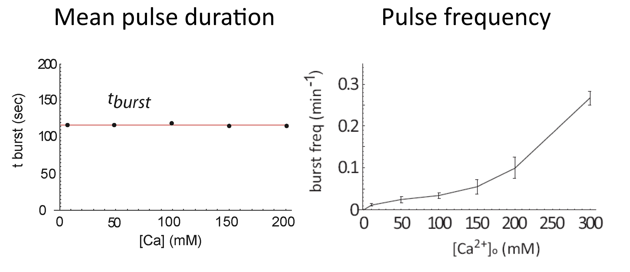
Average of Crz1 pulse dynamics in 42 cells, from L. Cai et al. (Nature, 2008)
In fact, even as pulse frequencies change dramatically, the entire distribution of pulse durations is apparently unaffected by the level of calcium:
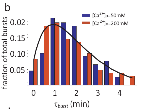
Distribution of pulse durations, from L. Cai et al. (Nature, 2008).
And we see a similar behavior at the level of pulse clusters, with calcium modulating their frequency, but not their mean duration. To extract these features, one first notes that the autocorrelation function is well fit by a sum of two exponentials with different timescales, corresponding to individual pulses and pulse clusters:
\begin{align} C_a = A_1 \mathrm{e}^{- \left(\frac{t}{\tau_{pulse}}\right)} + A_2 \mathrm{e}^{-\left(\frac{t}{\tau_{cluster}}\right)} \end{align}
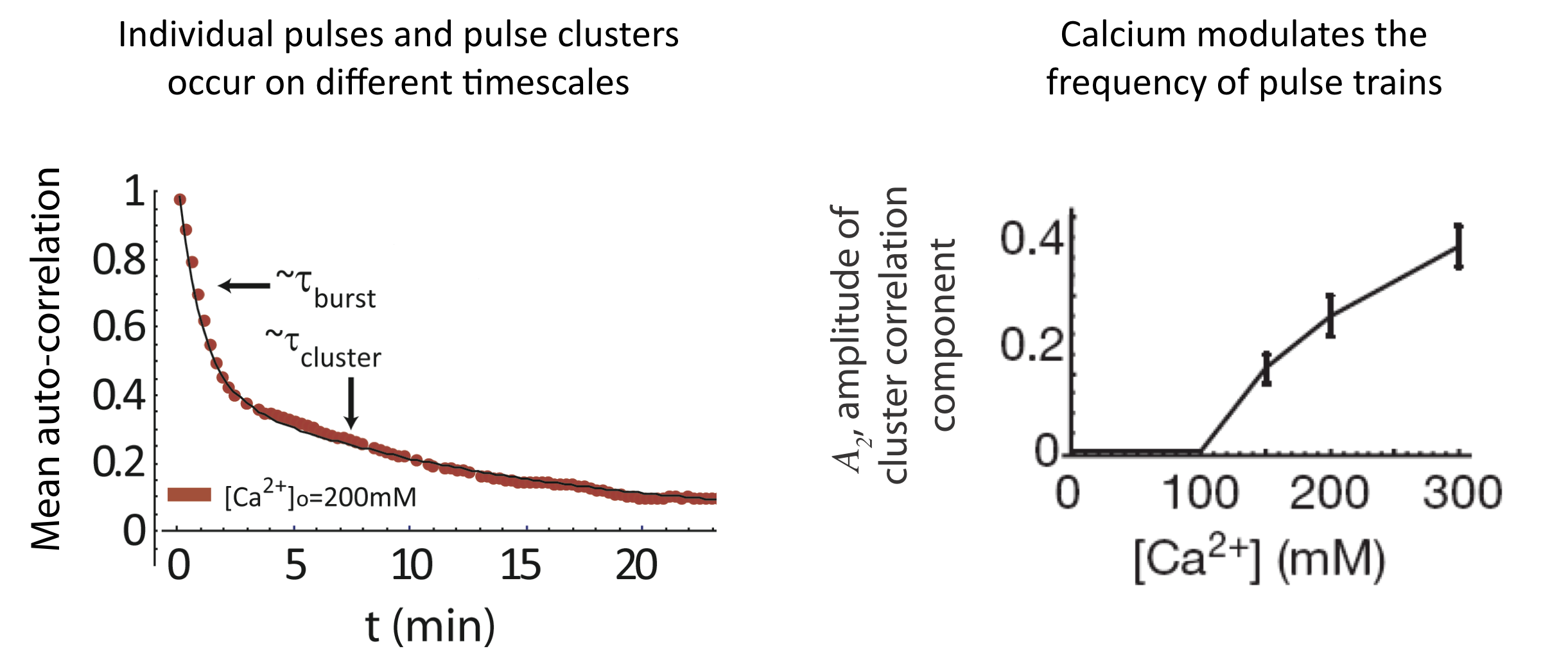
Analysis of pulse trains, from L. Cai et al. (Nature, 2008).
Finally, the initial response to calcium does not occur in all cells, but the fraction of cells that exhibit that response is also modulated by calcium:
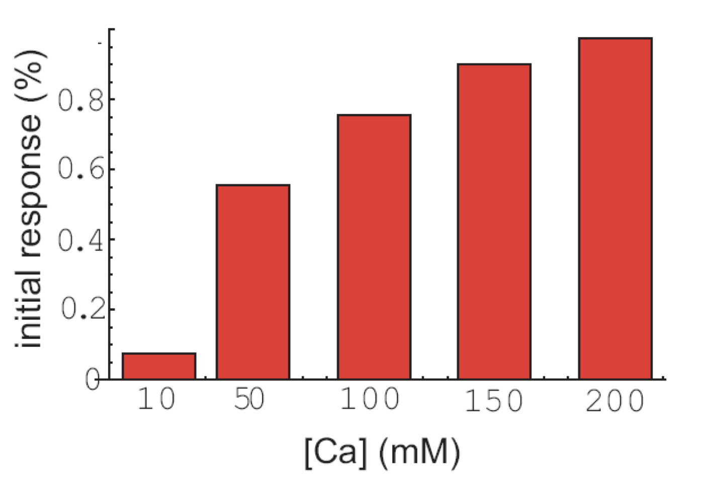
Analysis of pulse trains, from L. Cai et al. (Nature, 2008).
To summarize, calcium seems to modulate the frequency of individual pulses, pulse clusters, and even the appearance of initial responses, while not affecting the amplitude or duration of the same features!
How do we get the observed autocorrelation?
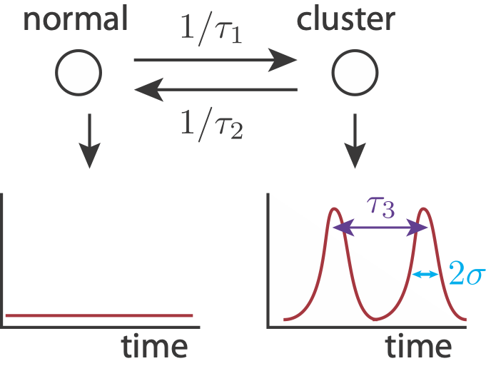
To show how pulse trains might give the observed biexponential mean autocorrelation function, we can build a simulated signal. We use the following simplified model. A cell can either be in a cluster state, in which it may have pulsed localization, or out of a cluster state, in which no localization occurs. Entry into a cluster state is a modeled as a Poisson process with time constant \(\tau_1\), and exit from a cluster state is modeled as a Poisson process with time constant \(\tau_2\). While in a cluster state, we may get localization events, also modeled as a Poisson process, with time constant \(\tau_3\). We model each pulse as a Gaussian-like peak in time with width \(2\sigma\). Finally, there is also noise in the signal.
First, we’ll code up some function to make our signal.
[6]:
def pulse_times(tau_1, tau_2, tau_3, t_max):
    t_pulse = []
    t = 0

    while t < t_max:
        # Wait for pulsing to turn on
        t += np.random.exponential(tau_1)

        # How long will pulsing last?
        t_end = t + np.random.exponential(tau_2)

        # Make pulses
        while t < t_end:
            t += np.random.exponential(tau_3)
            t_pulse.append(t)

    return np.array(t_pulse)


def pulse_signal(
    pulse_times,
    base_signal,
    pulse_amplitude,
    pulse_amplitude_sigma,
    noise_amplitude,
    sigma,
    t_max,
    n_samples,
):
    t = np.linspace(0, t_max * (1 + 0.02), n_samples)
    signal = base_signal + np.random.normal(0, noise_amplitude, len(t))
    for tp in pulse_times:
        signal += (
            pulse_amplitude
            * np.random.normal(1, pulse_amplitude_sigma)
            * st.norm.pdf(t, tp, sigma)
        )

    return t, signal


def make_signal(
    tau_1,
    tau_2,
    tau_3,
    base_signal,
    pulse_amplitude,
    pulse_amplitude_sigma,
    noise_amplitude,
    sigma,
    t_max,
    n_samples,
):
    t_pulse = pulse_times(tau_1, tau_2, tau_3, t_max)

    return pulse_signal(
        t_pulse,
        base_signal,
        pulse_amplitude,
        pulse_amplitude_sigma,
        noise_amplitude,
        sigma,
        t_max,
        n_samples,
    )
Let’s generate a typical signal and see how it looks.
[19]:
t, signal = make_signal(
    tau_1=10,
    tau_2=12,
    tau_3=1,
    base_signal=0.5,
    pulse_amplitude=1.5,
    pulse_amplitude_sigma=0.1,
    noise_amplitude=0.1,
    sigma=0.25,
    t_max=5000,
    n_samples=65536,
)

p = bokeh.plotting.figure(
    width=500,
    height=250,
    x_axis_label="time (min)",
    y_axis_label="nuclear fluorescent intensity (a.u.)",
)
p.line(t, signal, line_join="bevel")
bokeh.io.show(p)
We see clusters of nuclear localization separated by relatively quiet periods.
We will now generate many of these signals (100 of them) and compute the mean autocorrelation function.
[21]:
auto_corrs = np.empty((100, 4096 // 2))
for i in range(100):
    _, signal = make_signal(
        tau_1=100,
        tau_2=12,
        tau_3=1,
        base_signal=0.5,
        pulse_amplitude=1.5,
        pulse_amplitude_sigma=0.1,
        noise_amplitude=0.1,
        sigma=0.25,
        t_max=500,
        n_samples=65536,
    )

    tau, auto_corrs[i] = correlate(signal, signal, half=True)

mean_autocorr = np.mean(auto_corrs, axis=0)

p = bokeh.plotting.figure(
    width=400,
    height=250,
    x_axis_label="τ (min)",
    y_axis_label="autocorrelation",
    x_range=[-2, 50],
)
p.line(tau, mean_autocorr)
p.circle(tau, mean_autocorr)

bokeh.io.show(p)
---------------------------------------------------------------------------
ValueError                                Traceback (most recent call last)
<ipython-input-21-d4cd331611a4> in <module>
     14     )
     15
---> 16     tau, auto_corrs[i] = correlate(signal, signal, half=True)
     17
     18 mean_autocorr = np.mean(auto_corrs, axis=0)

ValueError: could not broadcast input array from shape (32768,) into shape (2048,)
Here, we see two decay timescales, a faster one corresponding to the typical width of individual pulses, and a longer one corresponding to the duration of pulse clusters.
When trying to validate data analysis approaches, it can be helpful to generate ‘synthetic data’ with known properties and then see how well the analysis captures those properties.
Why FM pulsing?
These observations provoke the natural question: Why use FM pulsing instead of a seemingly simpler continuous regulation system?
In non-biological contexts, FM or pulsatile regulatory systems offer a number of advantages compared to their AM counterparts:
FM radio is less susceptible to transmission noise that predominantly affects signal amplitude.
In neurobiology, transmission of signals through all or none spikes (action potentials) could allow signal propagation with minimal degradation.
“Bang bang” control systems work by regulating the fraction of time that a system is “on” rather than modulating its level of activity. Bang bang provides simple, intrinsically linear control, and does not require detailed knowledge of the exact input-output behavior of the device. One example where this scheme has been used is rocket thrusters. (A fun example of this is the classic lunar lander video game, in which one uses bang bang control to safely land a spacecraft: http://moonlander.seb.ly/).
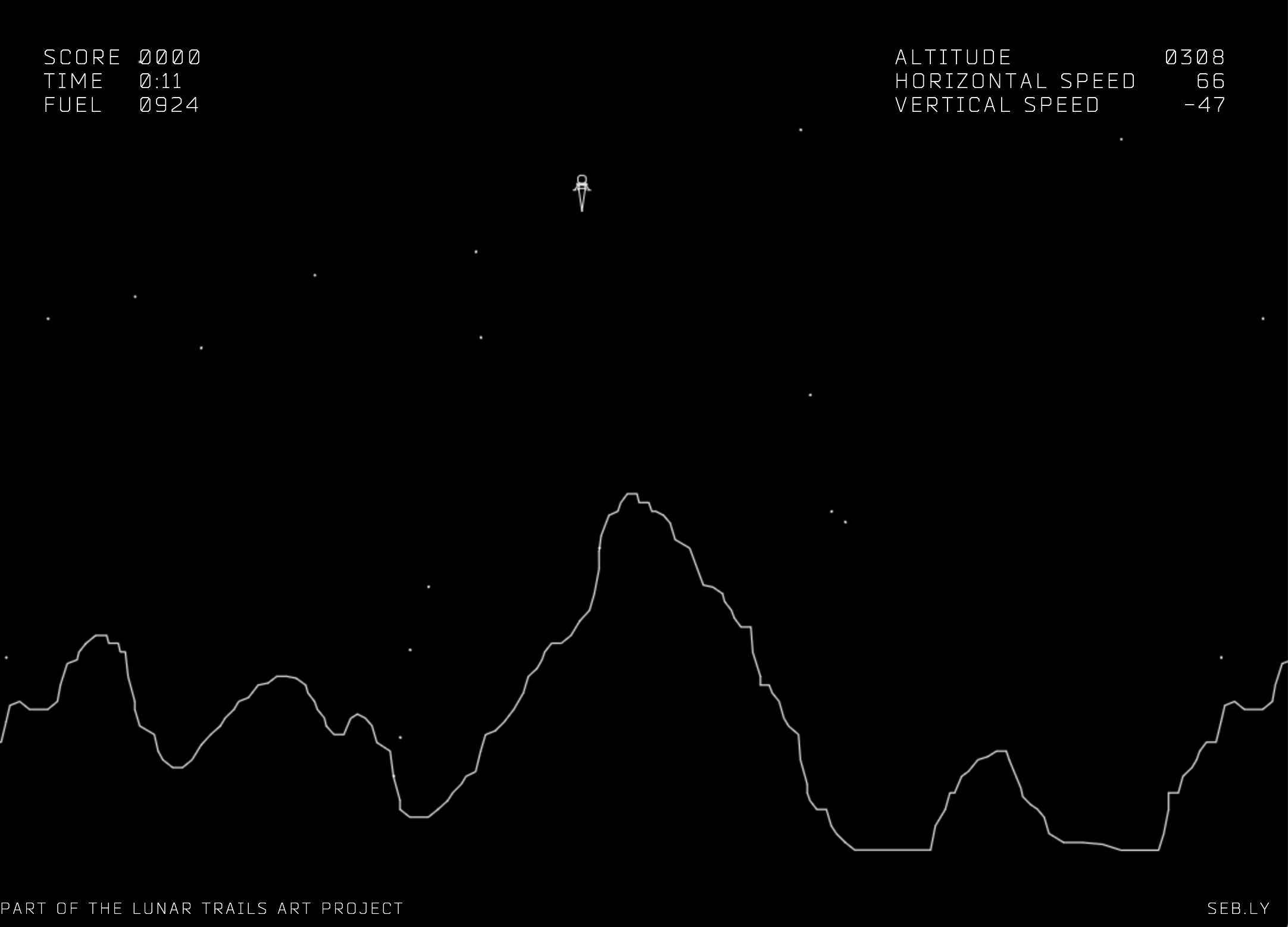
Moonlander screenshot; see http://moonlander.seb.ly/.
Which, if any, of these possible explanations might be relevant for the cell? As we will see, the third example—bang bang control—could provide insight into some of the benefits of FM pulsing.
FM, but not AM, regulation allows coordinated activation of diverse target genes
To think about the different effects of AM and FM-pulse regulation, we consider two hypothetical target genes that have different response functions to Crz1.
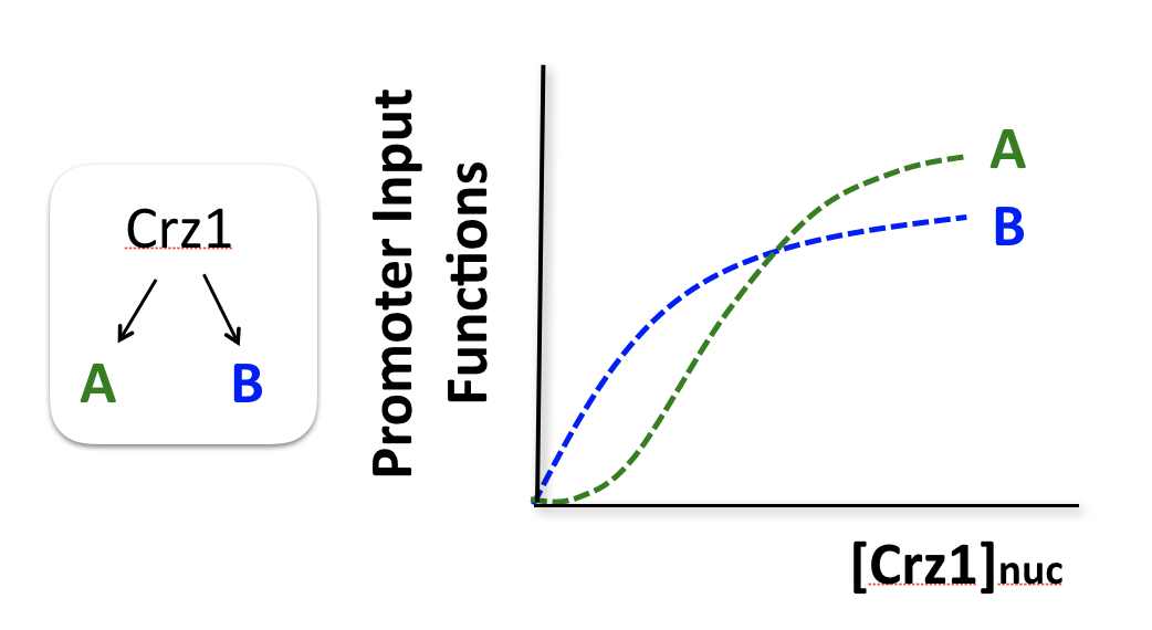
Consider two hypothetical Crz1 target genes with different response functions. These targets might have different sensitivities, different amplitudes, and different EC50s with respect to nuclear Crz1 concentration. Let’s imagine how these genes would respond to different levels of nuclear Crz1.
In an AM regulation system, low and high input levels produce different ratios of A and B expression. As illustrated here, low levels of nuclear Crz1 might produce more of B than of A. Higher levels of Crz1 would move one to the right on the response functions, generating more of both proteins, but shifting the ratio, so that A is now produced at a higher rate than B. In this sense, the ratio of A production to B production depends on the precise concentration of Crz1 in the nucleus.

Now contrast this behavior with what one might expect in the FM pulsing system. Here, increasing input level produces a higher frequency of pulses, but the durations and amplitudes of the pulses are not affected. Therefore, the ratio of A to B expression produced by each pulse (or the distribution of those ratios) remains the same regardless of the mean Crz1 activity. As a result, frequency modulation can vary both A and B expression in concert, maintaining a constant A to B ratio across a wide range of expression levels:
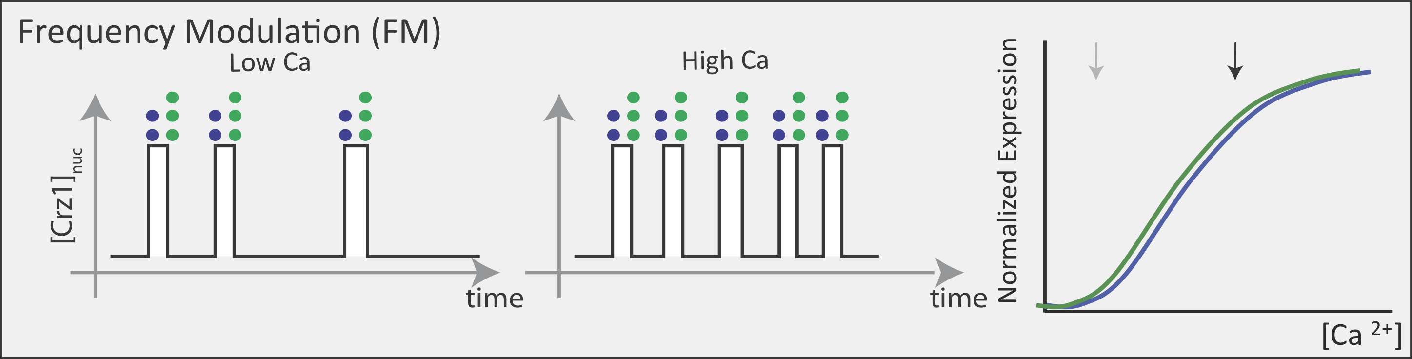
More generally, if we consider many target genes, one can see that FM pulsing ensures they are all co-regulated in fixed proportions, despite differences in their individual input functions.
These considerations suggest a simple design principle: FM pulsing enables coordinated regulation of diverse target genes.
Crz1 target genes show coordinated regulation
Does the real system in fact exhibit coordination regulation of its targets? If so, one would certainly expect to see target expression track pulse frequency. In fact, that does seem to occur:
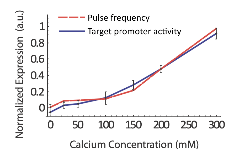
From L. Cai et al. (Nature, 2008).
More generally, we would expect that changing key parameters of the reporter would preserve this relationship. To check this, we constructed synthetic Crz1 target promoters with different numbers of binding sites (CDREs) for Crz1. The mean activity of these promoters varied over a 450-fold range.
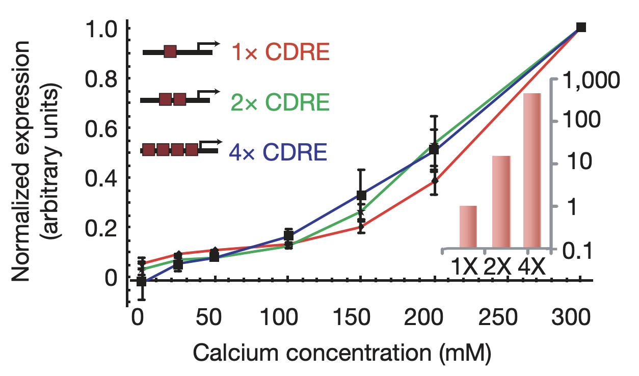
Synthetic target promoters show coordinated regulation. Synthetic promoters varying over 450-fold in their mean activity (inset) produce similar dose-response curves. From L. Cai et al. (Nature, 2008).
Furthermore, the same coordination can be observed with natural genes. The following plots show how diverse Crz1 target genes (black) compare to pulse frequency (red) in their response to calcium dose.
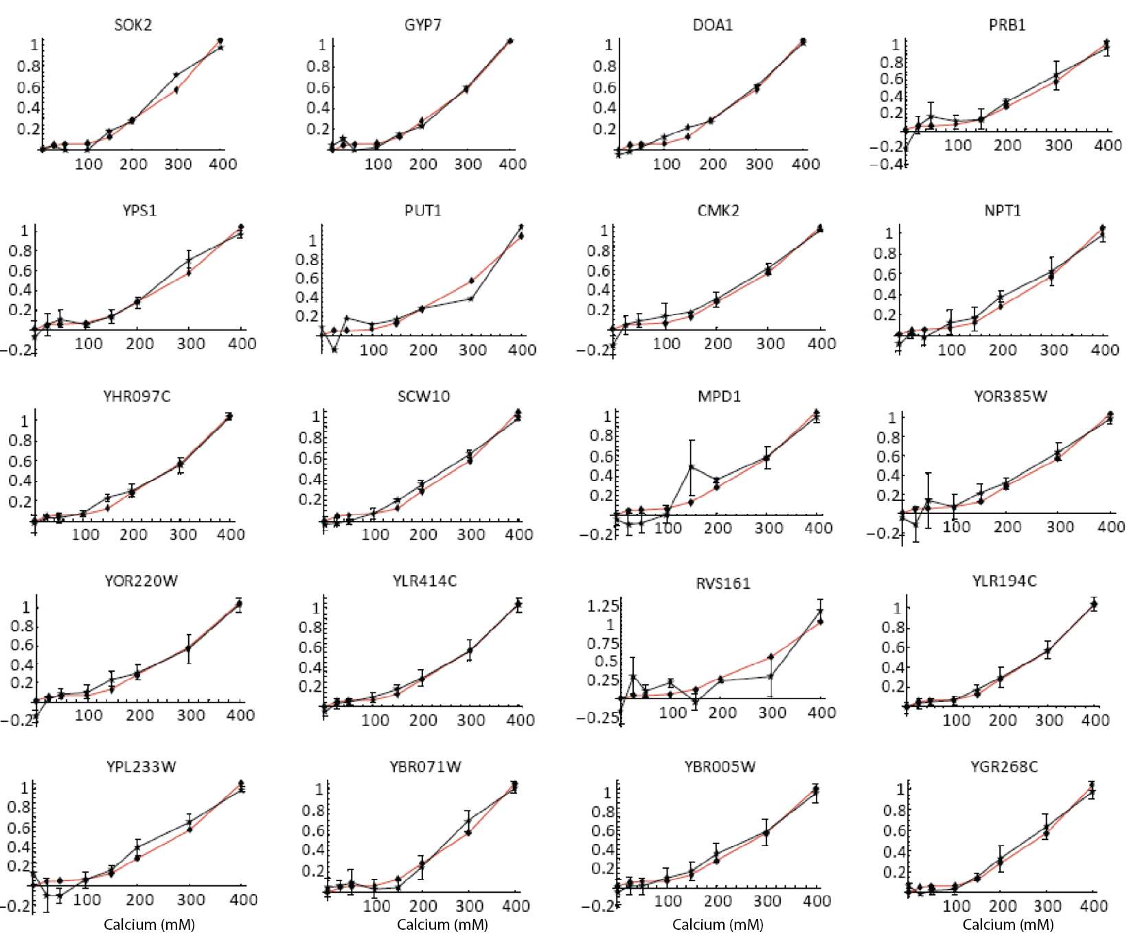
Natural target genes (black) and pulse frequency (red) show similar responses to calcium dose. From L. Cai et al. (Nature, 2008). Additional targets shown in paper.
What about “fine-tuning?”
In a fine-tuned model, all the promoters have the same dependence on Crz1 concentration, at least up to a scale factor for each promoter. That is, \(P_i\)(Crz1) \(= \alpha_i P_0\)(Crz1), where the index \(i\) labels each target promoter and \(P_0\) refers to a reference promoter.
If this were the case, then increasing the concentration of Crz1 should change all promoters to the same extent. Contrary to this expectation, experiments revealed that different promoters were affected to differing extents by Crz1 overexpression, suggesting that the observed coordination results from FM pulsing rather than from fine-tuning of target promoters.
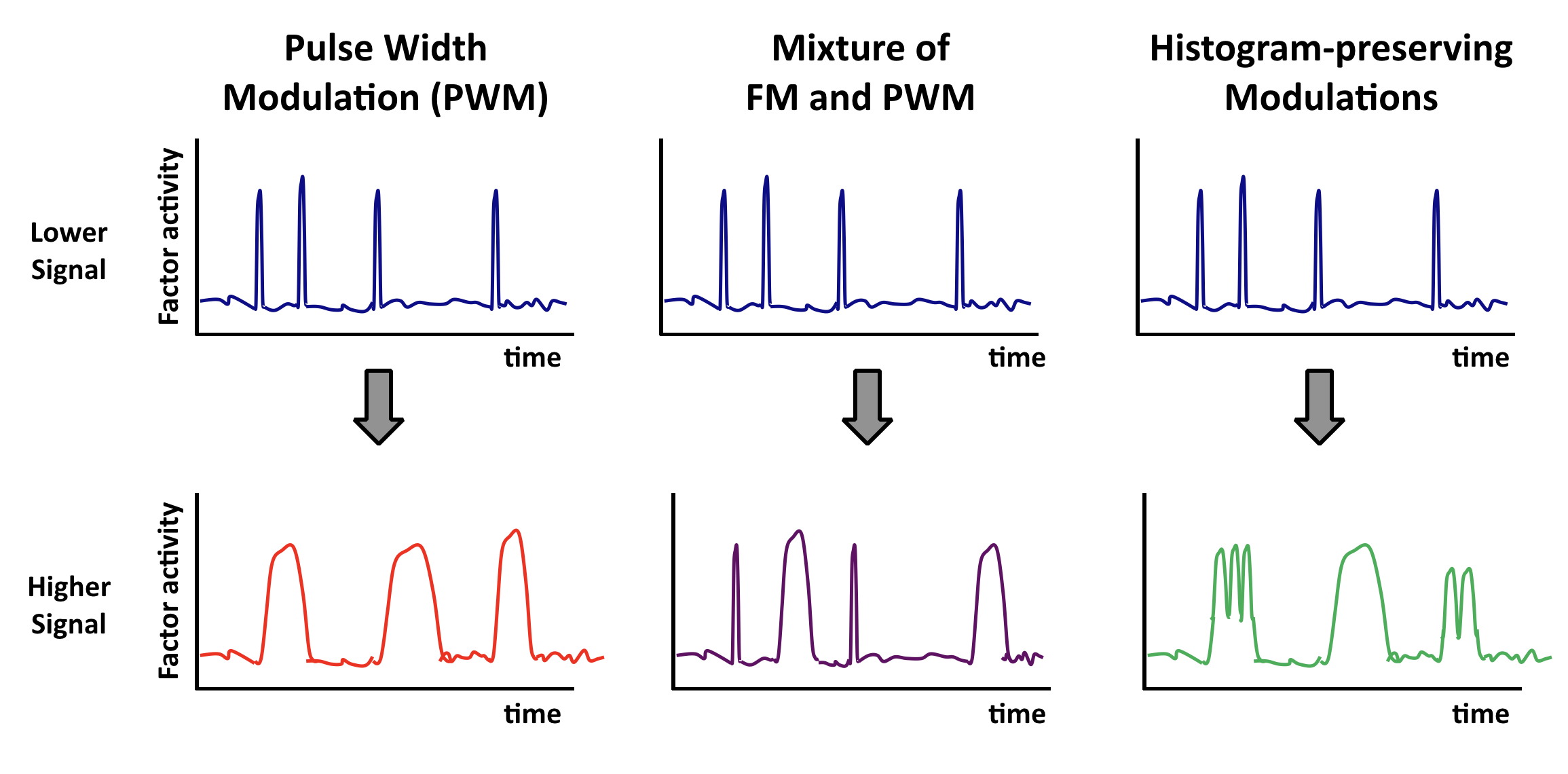
Other “histogram-preserving” modulations can also enable coordination.
Coordination can occur with multiple types of time-based regulation. It does not require frequency modulation per se. Any “histogram preserving” modulation in which input signals control only the fraction of time the factor spends in a distribution of ‘high’ states, but not the distribution of activities in either the low or high activity states, should work.
Here are some examples. In each case, top and bottom illustrations show, schematically, how time traces would be affected by a change in input.
Multiple pulsers: from frequency to phasing
So far we have focused on a single transcription factor, pulsing away in a single condition. But in reality there are likely to be multiple pulsatile transcription factors operating in the same cell at the same time, and potentially co-regulating many common target genes, something like this:
This leads to the next question: how do multiple pulsatile systems interact in time to control targets? Could cells use relative timing or phasing of dynamics between different transcription factors to control target genes in new ways?
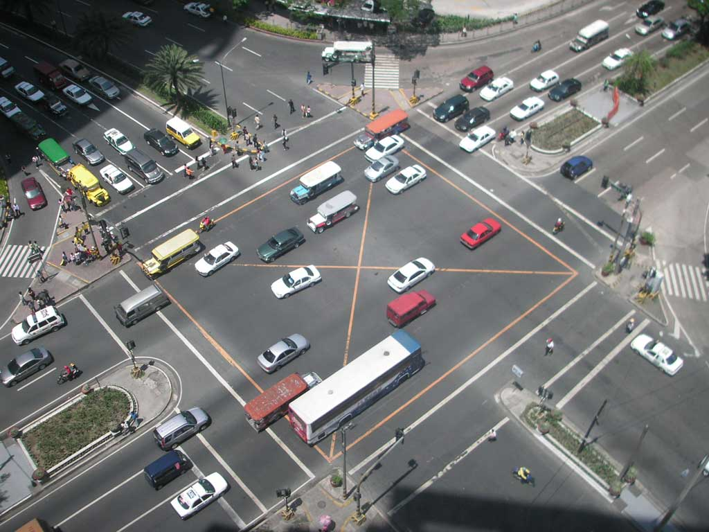
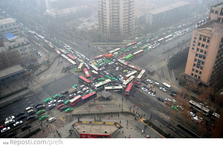
Phasing matters
The relative timing, or phasing, of different events – say, stoplights – can make a big difference in many contexts. What about the relative timing of pulses of different transcription factors in the same cell?
Msn2 and Mig1 pulse and co-regulate common target genes
Msn2 and Mig1, two major transcription factors in yeast, respond to overlapping stresses, including glucose limitation, and co-regulate some common target genes:
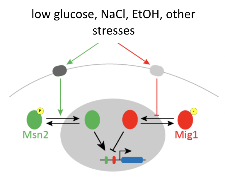
Msn2 is an activator, while Mig1 is generally a repressor.
You can imagine that if only Msn2 is present, it can easily activate the gene, but if both Msn2 and Mig1 are simultaneously present, it is a bit like stepping on both the accelerator (Msn2) and brake (Mig1) at the same time. If you do that, ideally, the brake will dominate and the car (target gene), will not move (activate).
Three-color strains enable simultaneous analysis of two transcription factors and one target
To be able to visualize Msn2 and Mig1 dynamics, along with their effects on a target gene, Y. Lin et al. (Nature, 2105) engineered a three color reporter system in yeast.
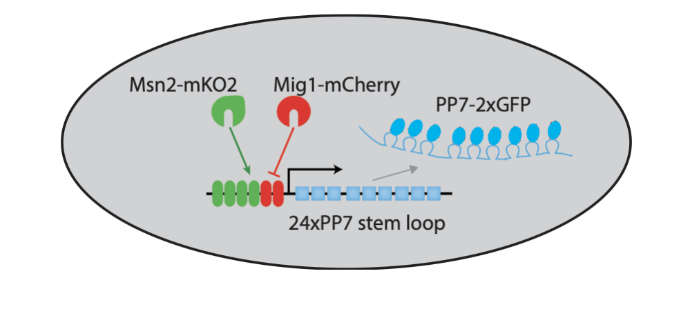
In this system, Msn2 and Mig1 are fused to distinct fluorescent protein colors. In addition, the RNA-binding protein PP7, fused to a third fluorescent protein, enables rapid and direct tracking of target transcription from synthetic and natural target genes; see Larson, et al. (Science, 2011).
Different inputs activate with different relative timing
In these movies, we can see that exposure of cells to either salt or ethanol each activate both transcription factors. However, they do so with different relative timing, either “out of phase” or “in phase”. Because M
For example, in this movie note that adding NaCl causes a sequential activation (nuclear localization) of Msn2 followed by Mig1, leading to increase in target expression.
By contrast, here we can see that adding ethanol to the same cells causes simultaneous activation (nuclear localization) of Msn2 and Mig1, producing little or no expression of the target:
These movies can be summarized with this plot:
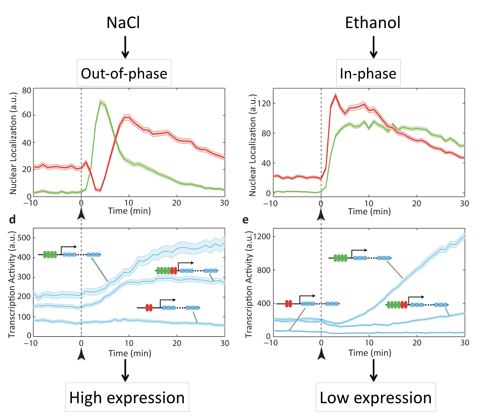
Different stresses activate Msn2 and Mig1 with different relative timing, resulting in distinct target activation patterns. The three target genes in each case so a full combinatorially regulated target as well as controls lacking one or the other set of binding sites. See Lin et al, Nature, 2015.
What we can see here is amazing: Different inputs activate the same transcription factors with different relative timing and this in turn determines whether target genes are activated or not.
Relative timing can be continuously modulated by glucose concentration
Another way to modulate this system is to vary glucose concentration. If one then tracks the dynamics of the two transcription factors, and computes the cross-correlation functions, one can see the relative amplitude of in phase and out of phase peaks gradually shifting:
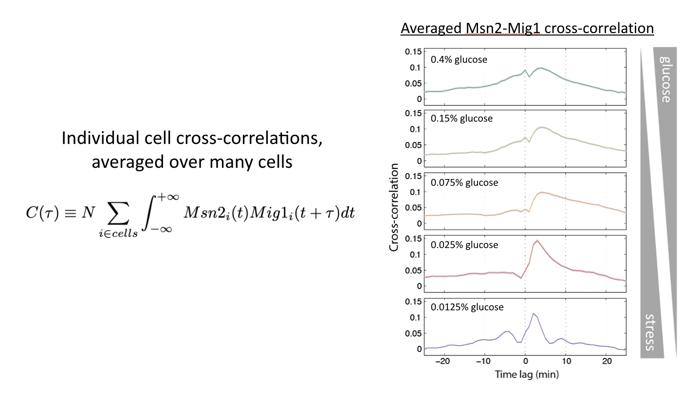
Glucose concentration determines relative timing of Msn2 and Mig1 pulses. See Lin et al, Nature, 2015.
This shows us that cells can and do encode signals not only in the overall dynamics of a single transcription factor but more generally in the relative timing of multiple transcription factors.
Imagine if we could somehow image the dynamic responses of all regulators in the same cell over time, while also observing their targets. It would be like hearing a whole symphony at once, rather than just a couple of instruments at a time. Perhaps we could gain a better understanding of how the dynamics of many regulators play out in time to control the cell.
Conclusions
Today we have seen that cells are organized not only in space but also in time. Perhaps we should not be surprised: just as electrical circuits have long made use of the time domain for complex regulation, so too do living cells. While we have examined a few core regulatory systems in yeast, similar types of dynamic regulatory strategies are likely to be quite general across pathways, cell types, and species.
To recap:
Time-based regulation provides a unique regulatory capability: controlling a diverse set of target genes in fixed proportions.
This capability is ideal for ensuring that protein products of multiple targets need to work together in fixed stoichiometries. At the same time, it may also be interesting to think about cases in which coordination is not desired. For example, when it is more optimal to trigger qualitatively distinct responses to high levels of input compared to low ones.
In some systems, inputs regulate target genes by regulating the relative timing with which multiple transcription factors activate.
Computing environment
[9]:
%load_ext watermark
%watermark -v -p numpy,scipy,bokeh,jupyterlab
Python implementation: CPython
Python version       : 3.8.8
IPython version      : 7.22.0

numpy     : 1.20.1
scipy     : 1.6.2
bokeh     : 2.3.1
jupyterlab: 3.0.14