18. Paradoxical regulation in intra- and intercellular circuits¶

Design principles

Futile cycles in kinase systems can linear amplification that is robust to total protein copy numbers.
Biphasic control can be accomplished with paradoxical regulation.

Concepts

Paradoxical regulation
Cellular circuits are necessarily autocatalytic

Techniques

Use of conservation laws can greatly simplify analysis.
Plotting phase portraits with a separatrix

[1]:

# Colab setup ------------------
import os, sys, subprocess
if "google.colab" in sys.modules:
    cmd = "pip install --upgrade biocircuits watermark"
    process = subprocess.Popen(cmd.split(), stdout=subprocess.PIPE, stderr=subprocess.PIPE)
    stdout, stderr = process.communicate()
# ------------------------------

import numpy as np
import scipy.integrate

import biocircuits

import bokeh.io
import bokeh.plotting

# Toggle for fully interactive plots
fully_interactive_plots = False
notebook_url = "localhost:8888"

bokeh.io.output_notebook()

Loading BokehJS ...

Paradoxical regulation: The I1-FFL revisited¶

Let us look back for a moment at an early chapter in which we considered an incoherent feed-forward loop, the I1-FFL, shown below, left. We can abstract the I1-FFL further, wherein X can activate Z and also repress Z with a delay, as shown below, right. The delay is due to the indirect nature of the repression of Z, having to do though the Y intermediary.

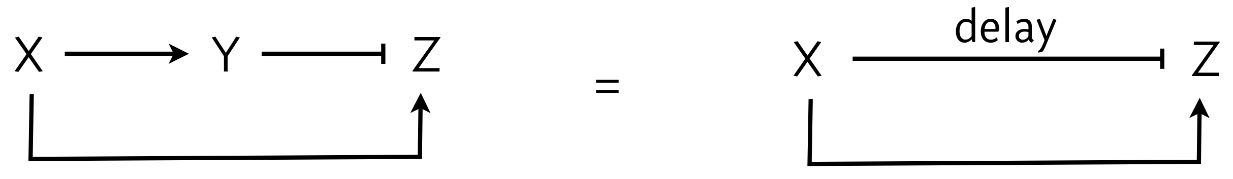
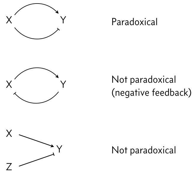
In looking at the figure to the right, we see that X both activates and represses Z. We say that X’s action on Y is paradoxical, in that the same gene has opposite regulatory effects on the same target. This stands in contrast to negative feedback loops or two different genes regulating the same target in opposite ways.

We have already seen properties of the I1-FFL with AND logic.

It is a pulse generator.
It has an accelerated response compared to an unregulated circuit.

In this lesson, we will further explore properties of circuits that employ paradoxical regulation, starting with simple two-component signaling circuits like the one shown above.

Two-component paradoxical circuits¶

Two-component circuits are ubiquitous in signaling systems. It makes sense that this is the case; we need minimally two components, a receptor and a signaling molecule (usually a conjunction with a kinase or phosphatase).

Input-output relationships generally depend on the concentrations of circuit components¶

Before considering a circuit with paradoxical regulation, let us first consider a simpler circuit wherein a signaling molecule allows the receptor kinase X to phosphorylate of a signaling molecule Y, as shown below.

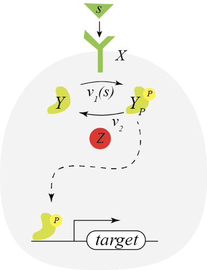
If we assume the enzymes operate at saturation, we have

\begin{align} \frac{\mathrm{d}y_p}{\mathrm{d}t} = v_1(s)\,x \, y - v_2\,z \, y_p. \end{align}

We also have conservation of mass; defining \(y_0\) to be the total concentration of Y, we have \(y_0 = y + y_p\). Using this expression, we have

\begin{align} \frac{\mathrm{d}y_p}{\mathrm{d}t} = v_1(s)\,x \, (y_0-y_p) - v_2\,z \, y_p. \end{align}

We can solve for the steady state concentration of phosphorylated Y, which will affect the expression of the target gene, by setting \(\mathrm{d}y_p/\mathrm{d}t = 0\) and solving. The result is

\begin{align} y_p(s) = \frac{v_1(s)\,x}{v_1(s)\,x + v_2\,z}\,y_0. \end{align}

This expression reveals a limitation of this circuit. The amount of \(y_p\) is obviously dependent on the amount of X, total amount of Y, and amount of Z. Since noise limits the precision with the systems own components can be controlled, we might prefer the amount of \(y_p\) to depend only on the concentration of the signaling molecule, \(s\), and to be robust to the concentrations X, Y, and Z are around.

A paradoxical two-component signaling system is robust to variation in its own components¶

Now consider instead a situation where the receptor X is a bifunctional kinase. In its phosphorylated form, it phosphorylates Y via phosphotransfer with rate \(v_3\). This is its activating regulation. In its dephosphorylated state, it serves to dephosphorylate Y with rate \(v_2\), giving it its paradoxical repressive regulation. So, X paradoxically has both kinase (phosphotransfer) and phosphatase (dephosphorylation) activity on the same substrate protein, Y. It also gets phosphorylated in contact with the signaling molecules S through consumption of an ATP. This circuit consumes energy by phosphorylating and dephosphorylating the same substrate, “undoing its own activity” in what is referred to as a futile cycle.

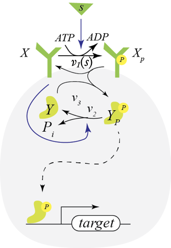
We can write out the full dynamics of this system and solve for the steady state, but we can take a shortcut. We can think of the system a black box that takes in ATP and outputs ADP and inorganic phosphate. A phosphate comes in as part of ATP and goes out as inorganic phosphate.

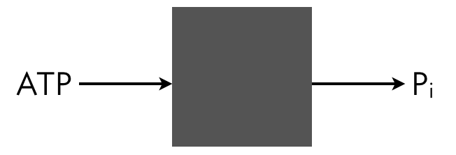
Conservation of mass dictates that the total flux of this phosphate into the system must match the total flux of Pᵢ out of the system. The influx is \(v_1(s)\,x\) and the outflux is \(v_2\,x\,y_p\). Setting these fluxes to be equal gives

\begin{align} v_1(s)\,x = v_2\,x\,y_p, \end{align}

so that

\begin{align} y_p = \frac{v_1(s)}{v_2}. \end{align}

This actually is not quite complete, since we still need to respect conservation of mass of Y, so

\begin{align} y_p = \begin{cases} \frac{v_1(s)}{v_2} & y_0 \ge \frac{v_1(s)}{v_2},\\[1em] y_0 & y_0 < \frac{v_1(s)}{v_2}. \end{cases} \end{align}

This is dependent only on \(s\), and is completely independent of the total amounts of the proteins X and Y. Importantly, the activity, as quantified by the concentration of phosphorylated Y, is linear in the input \(v_1(s)\), with a slope of \(v_2^{-1}\). Thus, this system, at least before saturating, is a perfect linear amplifier of the input signal.

Key to the linear amplification of signal is the following.

The cell must produce enough Y to make sure it does not saturate. That is, \(y_0\) must be at least \(v_1(s_\mathrm{max})/v_2\), where \(s_\mathrm{max}\) is the maximum expected concentration of the signaling molecule.
The gain of the amplifier (the slope of the linear response) is inversely proportional to the dephosphorylation rate \(v_2\). Slow dephosphorylation gives a larger gain.
It is critical that only the dephosphorylated state of the bifunctional kinase X have phosphatase activity. (If the phosphorylated state could act as a phosphatase, the inorganic phosphate balance changes, and we lose the linear amplification feature.)
All enzymes are operating at saturation. We would lose perfect linear amplification due to nonlinearities if they were not.
We are neglecting slow reactions, such as spontaneous dephosphorylation, which would also destroy robustness to total protein levels.

An example paradoxical signaling system¶

The EnvZ-OmpR system in E. coli is a classic system that features a bifunctional kinase with paradoxical signaling. It has the same architecture as our example above. EnvZ is a histidine kinase that senses osmotic stress, and OmpR regulates expressin of porin genes in response to osmolarity.

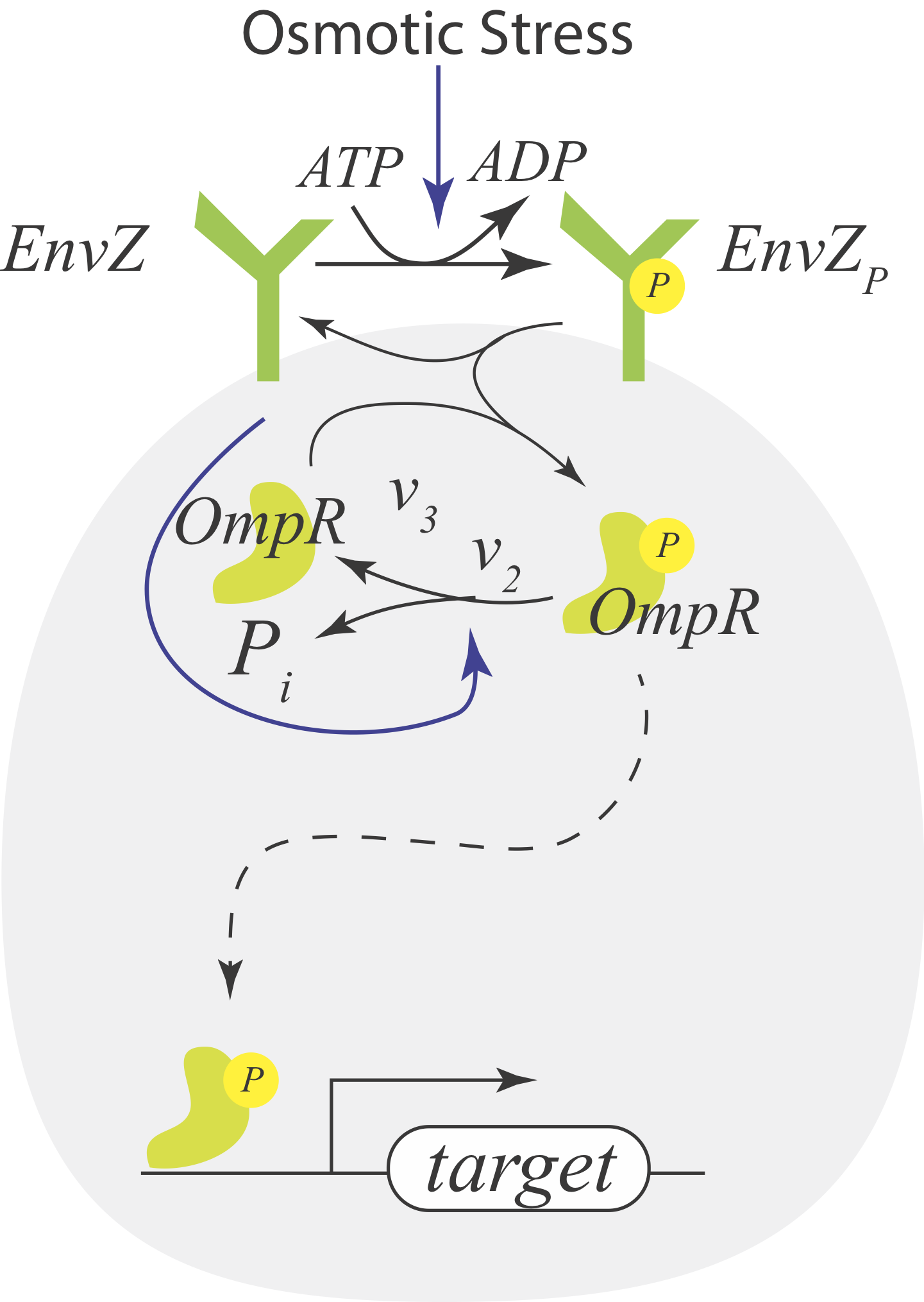
Batchelor and Goulian (PNAS, 2003) introduced a plasmid to E. coli cells where OmpR is under control of the lac promoter. They then adjusted the OmpR levels by titrating IPTG and monitored expression of a fluorescent reporter protein expressed from a target promoter. The compared target promoter activity at low osmolarity (in a minimal medium) and at high osmolarity (minimal medium with 15% sucrose). The result of their experiment is shown below (using data digitized from the paper).

[2]:

data_low = np.array(
    [
        [-0.9731, 0.5020],
        [-0.4584, 0.9084],
        [0.0087, 0.9920],
        [0.2800, 0.8486],
        [0.5300, 0.7171],
        [0.9079, 0.7649],
        [1.0654, 0.9084],
        [1.0996, 0.9920],
        [1.1593, 1.1116],
        [1.3748, 2.2709],
    ]
)

data_high = np.array(
    [
        [-0.9787, 0.2777],
        [-0.6626, 7.6505],
        [-0.1894, 11.3891],
        [0.2365, 11.5047],
        [0.2833, 11.5021],
        [0.4325, 12.1910],
        [0.6796, 12.5956],
        [0.9735, 12.9975],
        [1.0717, 15.0837],
        [1.1288, 29.1641],
    ]
)

p = bokeh.plotting.figure(
    frame_height=250,
    frame_width=450,
    x_axis_label="fold increase in OmpR",
    y_axis_label="target promoter activity (a.u.)",
    x_axis_type="log",
    y_axis_type="log",
)
p.circle(10 ** data_low[:, 0], data_low[:, 1], legend_label="low osmolarity")
p.circle(
    10 ** data_high[:, 0],
    data_high[:, 1],
    color="orange",
    legend_label="high osmolarity",
)
p.legend.location = "center"
bokeh.io.show(p)

Astoundingly, over at least an order of magnitude the target promoter activity is robust to OmpR concentration, sensitive only to the osmolarity of the surrounding environment.

Design considerations for two-component paradoxical signaling¶

At the heart of linear amplification by two-component signaling is the bifunctional histidine kinase (labeled X in our generic two-component signaling system). The total concentration X affect the rates of all reactions. Too little X results in a slow response time, but too much X squanders cellular resources. So, there is some optimization with respect to the amount of X, depending on the cell’s needs. Importantly, if all enzymes are operating at saturation, and the response is fast enough that we can continue to neglect slow reactions like spontaneous phosphorylation, the perfect linear amplification at steady state is robust to the total level of X (and also Y).

Cellular circuits¶

So far, we have mostly been considering circuits of genes and their products within single cells. Like genes, cells can form circuits, called cellular circuits. We started discussing cellular circuits when we discussed bet hedging, and we will now consider this more formally.

In general, a cellular circuit can involve three main types of interactions, depicted in the example circuit below.

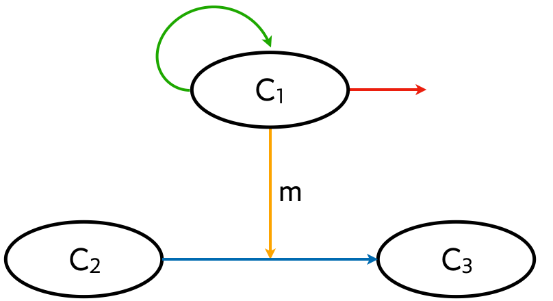
Proliferation (green arrow).
Secretion (orange arrow).
Differentiation (blue arrow).
Cell death (red arrow).

In the example circuit, the secreted molecule m affects differentiation of cells of type 2 into those of type 3, but a secreted molecule in general may have any arbitrary effect on cellular behavior.

An important feature of cellular circuits is that they are necessarily autocatalytic in that cells are necessary to proliferate. While the simplest model for gene expression, that of unregulated expression, was

\begin{align} \frac{\mathrm{d}x}{\mathrm{d}t} = \beta - \gamma x, \end{align}

where \(x\) is the concentration of the gene product, the simplest model for a cellular circuit, that of unregulated division and cell death has a different form,

\begin{align} \frac{\mathrm{d}x}{\mathrm{d}t} = \beta x - \gamma x, \end{align}

where \(x\) here is the concentration of cells. Note that the production term is linear in \(x\). There is only one steady state for this system, \(x = 0\). If \(\gamma > \beta\), the steady state is stable; the cells die out more rapidly than they can divide. However, if \(\beta > \gamma\), the cells grow without bound. Physically, \(\beta\) is a function of \(x\) as well, and saturates for large \(x\). In practice, there are many regulatory processes governing cell growth, and also death, and this leads to more stable nonzero steady states and interesting dynamics.

Cellular circuits abound, both in single-cell and multicellular organisms. Many of the circuits are paradoxical. For a nice discussion of possible paradoxical cellular circuits, see Hart et el., PNAS, 2012.

We now consider two cellular circuits with paradoxical components.

T-cell differentiation is controlled by cytokines¶

Hematopoietic stem cell differentiation is a classic example of a cellular circuit in higher organisms. Cells secrete a variety of cytokines, and the concentrations of the respective cytokines and ligands orchestrate differentiation. T-cell differentiation in the immune system, depicted below, is another example.

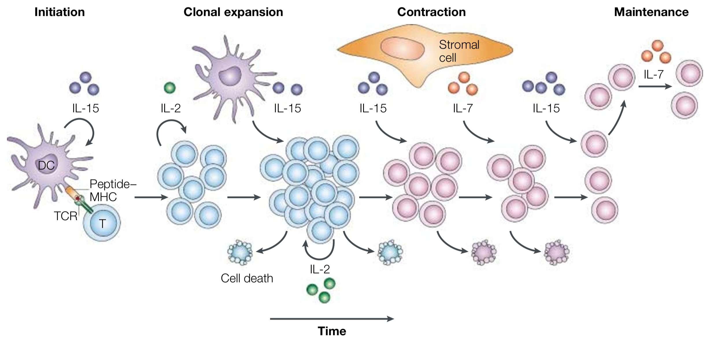
Image taken from Schluns and Lefrançois (Nat. Rev. Immun., 2003).

As the T-cell response is initiated when a T-cell receptor (TCR) comes in contact with a major histocompatibility complex (MHC) molecule, the cytokine interleukin-15 (IL-15) is secreted to activate dendritic cells (DCs). Clonal expansion of T-cells follows, regulated by IL-2. Other interleukin cytokines are involved in the contraction phase, and finally in the maintenance phase for long-term memory.

Importantly, prior to the contraction phase, a clonal population of activated T-cells must be maintained. It is thought that the circuit below serves to regulate the population size of active T-cells.

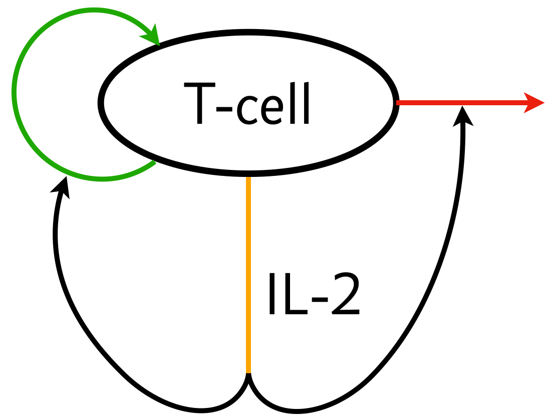
The T-cells can proliferate and excrete IL-2. IL-2, in term acts paradoxically to promote proliferation and also to promote T-cell death. In order to be effective in the context of the immune system, this circuit has the following design criteria.

The T-cell population must be homeostatic.
The T-cell population must be controllable.
There must be a stable off state. This enables T-cell deactivation.

This was examined in a paper by Hart and coworkers (Cell, 2014).

Biphasic control is a type of paradoxical circuit¶

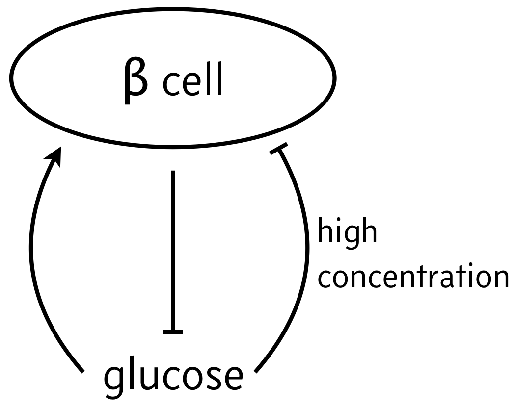
We now turn to a circuit featuring biphasic control of cell populations, in which a molecule is favorable for cell growth at moderate concentrations, but detrimental if in very small or very large concentrations. As a classic example of biphasic control, we can think of the relationship between β cells and glucose. In response to elevated glucose levels, β cells secrete insulin, which serves to reduce glucose levels. But if glucose levels get too high, it is toxic to the β cells, which can then die off. So, the propensity for β cells to produce insulin (simply noted “β cells” in the schematic below) is maximal at intermediate levels of glucose.

We will investigate the consequences of this circuit architecture in this lesson. In doing so, we will review many of the important techniques from dynamical systems in analyzing biological circuits. This analysis closely follows Karin and Alon, Molec. Sys. Biol., 2017.

Dynamical equations¶

We model the cellular circuit with a system of ODEs as follows.

\begin{align} \frac{\mathrm{d}c}{\mathrm{d}t} &= (\beta_c(m) - \gamma_c(m))\,c \\[1em] \frac{\mathrm{d}m}{\mathrm{d}t} &= \beta_m - \gamma_m(c)\,m. \end{align}

The production and degradation rate of insulin producing β cells are both dependent on the glucose concentration \(m\) and are proportional to the cell concentration \(c\). The parameter \(\beta_m\) is the feed rate of glucose, which is accomplished in an organism by eating and drinking, or in a cell culture by injection of glucose.

We choose the following forms for the functions above.

\begin{align} \beta_c(m) &= \beta_{c,1}\,\frac{(m/k_\beta)^{n_\beta}}{1 + (m/k_\beta)^{n_\beta}},\\[1em] \gamma_c(m) &= \gamma_{c,0} + \gamma_{c,1}\,\frac{(m/k_\gamma)^{n_\gamma}}{1 + (m/k_\gamma)^{n_\gamma}}, \\[1em] \gamma_m(c) &= \gamma_{m,1}\,c. \end{align}

The expression for \(\beta_c(m)\) describes saturating glucose-fed growth. The expression for \(\gamma_c(m)\) has two terms: baseline die-off \(\gamma_{c,0}\) and die-off due to too much glucose. Finally, the \(\gamma_m(c)\) term describes cellular consumption of glucose.

Importantly, in looking at the forms of \(\beta_c(m)\) and \(\gamma_c(m)\), we see that for small and large \(m\), the growth rate \(\beta_c(m) - \gamma_c(m)\) is negative, leading to decrease in insulin producing β cells. But for intermediate \(m\), we have positive \(\beta_c(m) - \gamma_c(m)\).

We can nondimensionalize, defining

\begin{align} &\beta_c = \frac{\beta_{c,1}}{\gamma_{c,0}},\\[1em] &\gamma = \frac{\gamma_{c,1}}{\gamma_{c,0}},\\[1em] &\kappa = \frac{k_\beta}{k_\gamma},\\[1em] &\beta_m \leftarrow \frac{\beta_m}{k_\beta \gamma_{c,0}},\\[1em] &t \leftarrow \gamma_{c,0}t,\\[1em] &m \leftarrow k_\beta m, \\[1em] &c \leftarrow \frac{\gamma_{c,0}}{\gamma_{m,1}}\,c. \end{align}

The result is

\begin{align} \frac{\mathrm{d}c}{\mathrm{d}t} & = \left(\beta_c\,\frac{m^{n_\beta}}{1 + m^{n_\beta}} - 1 - \gamma\,\frac{(\kappa m)^{n_\gamma}}{1 + (\kappa m)^{n_\gamma}}\right)c, \\[1em] \frac{\mathrm{d}m}{\mathrm{d}t} &= \beta_m - cm. \end{align}

These are the dynamical equations we will study.

Solving numerically¶

First, we’ll write functions necessary to perform the numerical integration. Note that we are using techniques of modular programming here; we write functions that do single simple tasks.

[3]:

def dc_dt(c, m, beta_c, gamma, kappa, n_beta, n_gamma):
    return (
        beta_c * biocircuits.act_hill(m, n_beta)
        - 1
        - gamma * biocircuits.act_hill(kappa * m, n_gamma)
    ) * c


def dm_dt(c, m, beta_m):
    return beta_m - c * m


def ode_rhs(x, t, beta_m, beta_c, gamma, kappa, n_beta, n_gamma):
    """Compute right-hand-side of pair of ODEs."""
    c, m = x
    return np.array(
        [dc_dt(c, m, beta_c, gamma, kappa, n_beta, n_gamma), dm_dt(c, m, beta_m),]
    )

Let’s integrate, and see what happens, starting at two different initial concentrations of cells , both with a dimensionless glucose level of 1/2. We take the parameter values from the Karin and Alon paper.

[4]:

# Specify parameters
beta_m = 3.79
beta_c = 16.0
gamma = 20.0
kappa = 0.875
n_beta = 6
n_gamma = 6

# Package for the integrating function
params_c = (beta_c, gamma, kappa, n_beta, n_gamma)
params_m = (beta_m,)
params = params_m + params_c

# Set up initial condition and solve
x0 = np.array([2, 0.5])
t = np.linspace(0, 3, 400)
x_low = scipy.integrate.odeint(ode_rhs, x0, t, args=params)

# And again with higher initial condition
x0 = np.array([5, 0.5])
x_high = scipy.integrate.odeint(ode_rhs, x0, t, args=params)

# Plot the result
p = bokeh.plotting.figure(width=450, height=300, x_axis_label="time")
p.line(t, x_low[:, 0], line_width=2, legend_label="cells, low initial cell density")
p.line(
    t,
    x_low[:, 1],
    line_width=2,
    color="orange",
    legend_label="glucose, low initial cell density",
)
p.line(
    t,
    x_high[:, 0],
    line_width=2,
    line_dash="dashed",
    legend_label="cells, high initial cell density",
)
p.line(
    t,
    x_high[:, 1],
    line_width=2,
    color="orange",
    line_dash="dashed",
    legend_label="glucose, high initial cell density",
)
p.legend.location = "top_left"

bokeh.io.show(p)

When the number of β cells producing insulin is initially low (solid lines), the cells stop producing insulin and the glucose concentration grows to high levels, a “diabetes condition.” Conversely, when the number of β cells producing insulin is higher (dashed lines), they stabilize and maintain a consistent insulin level.

Plotting the phase portrait¶

We can solve for various parameter values, and can even make interactive plots where we vary initial conditions, but a phase portrait provides a concise view into the system dynamics from various starting points.

First, we will plot the flow of the dynamical system.

[5]:

c_range = [1, 7]
m_range = [0, 2]

p = biocircuits.phase_portrait(
    dc_dt,
    dm_dt,
    c_range,
    m_range,
    params_c,
    params_m,
    x_axis_label="c",
    y_axis_label="m",
    color="#e6ab02",
    plot_width=350,
)

bokeh.io.show(p)

Next, we add the nullclines. The \(m\)-nullcline is easy to compute. We solve

\begin{align} \frac{\mathrm{d}m}{\mathrm{d}t} = \beta_m - c m = 0, \end{align}

which gives

\begin{align} m = \frac{\beta_m}{c}. \end{align}

The \(c\)-nullcline is more challenging. We need to solve

\begin{align} \frac{\mathrm{d}c}{\mathrm{d}t} & = \left(\beta_c\,\frac{m^{n_\beta}}{1 + m^{n_\beta}} - 1 - \gamma\,\frac{(\kappa m)^{n_\gamma}}{1 + (\kappa m)^{n_\gamma}}\right)c = 0. \end{align}

An obvious solution is \(c = 0\). The means there is a vertical nullcline along the \(m\)-axis in the \(x\)-\(m\) plane. There may be horizontal lines (fixed \(m\), nonzero \(c\)) where

\begin{align} f(m) \equiv \beta_c\,\frac{m^{n_\beta}}{1 + m^{n_\beta}} - 1 - \gamma\,\frac{(\kappa m)^{n_\gamma}}{1 + (\kappa m)^{n_\gamma}} = 0. \end{align}

This can be rewritten as

\begin{align} \beta_c\,\frac{m^{n_\beta}}{1 + m^{n_\beta}} = 1 + \gamma\,\frac{(\kappa m)^{n_\gamma}}{1 + (\kappa m)^{n_\gamma}}. \end{align}

Both the right-hand-side and left-hand-side are monotonically increasing functions of \(m\). Each side also has a single inflection point and asymptotes to a finite value. The right-hand-side starts above the left-hand-side at \(m=0\). Therefore the lines represented by either side of this equation may cross zero, one, or two times, depending on the parameters. Therefore, there are either zero, one, or two horizontal lines in the \(c\)-nullcline.

To find the values of \(m\) for which we have a horizontal line for the \(c\)-nullcline, we need to find the roots of \(f(m)\). As is often the case with root finding, there are many ways to do it, and some work better than others. Our strategy here is to brute-force find the places where the \(f(m)\) curve crosses the \(m\)-axis by gridding up the axis and evaluating the sign of \(f(m)\) at each point. Wherever the sign changes, we know the function crossed the \(m\)-axis. We then hone in on the root near a crossing point using Brent’s method. We code this up below.

[6]:

def growth_rate(m, beta_c, gamma, kappa, n_beta, n_gamma):
    """Growth rate, f(m), of β cells"""
    return dc_dt(1, m, beta_c, gamma, kappa, n_beta, n_gamma)


def dc_dt_nullclines(m_range, beta_c, gamma, kappa, n_beta, n_gamma):
    """Determine values for horizontal nullclines."""
    # Brute force to guess how many roots
    m = np.linspace(m_range[0], m_range[1], 1000)
    sgn = growth_rate(m, beta_c, gamma, kappa, n_beta, n_gamma) > 0
    switches = np.where(np.diff(sgn))
    args = (beta_c, gamma, kappa, n_beta, n_gamma)

    # Hone in on each root
    return np.array(
        [
            scipy.optimize.brentq(growth_rate, m[i - 1], m[i + 1], args=args)
            for i in switches[0]
        ]
    )


def plot_nullclines(
    c_range, m_range, beta_m, beta_c, gamma, kappa, n_beta, n_gamma, p
):
    # dm/dt = 0 nullcline
    c = np.linspace(*c_range, 200)
    p.line(c, beta_m / c, line_width=2, color="#7570b3")

    # dc/dt = 0 nullcline
    m_vals = dc_dt_nullclines(m_range, beta_c, gamma, kappa, n_beta, n_gamma)
    for m in m_vals:
        p.ray(0, m, length=0, angle=0, line_width=2, color="#1b9e77")

    p.ray(0, 0, length=0, angle=np.pi / 2, line_width=2, color="#1b9e77")

    return p


# Add nullclines to the phase portrait
p = plot_nullclines(
    c_range, m_range, beta_m, beta_c, gamma, kappa, n_beta, n_gamma, p
)

bokeh.io.show(p)

Finding and characterizing fixed points¶

The fixed points are where the nullclines cross. Since we know the values of \(m\) for which the \(c\)-nullcline is horizontal (we found them numerically), we can use them to get the value of \(c\) for a fixed point via \(c = \beta_m/m\).

[7]:

def fixed_points(
    c_range, m_range, beta_m, beta_c, gamma, kappa, n_beta, n_gamma
):
    """Give all fixed points with a given range"""
    m = dc_dt_nullclines(m_range, beta_c, gamma, kappa, n_beta, n_gamma)
    c = beta_m / m

    return np.array([[c_val, m_val] for c_val, m_val in zip(c, m)])

In addition to finding the fixed points, we need to characterize them as being stable or unstable. To that end, we can perform a linear stability analysis. We expand the system of ODEs in a Taylor series about a fixed point \((c_0, m_0)\), keeping only terms to first order in the perturbations \(\delta m\) and \(\delta c\). Note that this means we do not keep terms of order \(\delta m \delta c\).

\begin{align} &\frac{\mathrm{d}\delta c}{\mathrm{d} t} = \left(\beta_c\,\frac{m_0^{n_\beta}}{1 + m_0^{n_\beta}} - 1 - \gamma\,\frac{(\kappa m_0)^{n_\gamma}}{1 + (\kappa m_0)^{n_\gamma}}\right)\delta c + c_0\left(\beta_c\,\frac{n_\beta m_0^{n_\beta-1}}{(1+m_0^{n_\beta})^2} - \gamma\,\frac{n_\gamma (\kappa m_0)^{n_\gamma}}{m_0(1+(\kappa m_0)^{n_\gamma})^2}\right)\delta m ,\\[1em] &\frac{\mathrm{d}\delta m}{\mathrm{d} t} = -m_0\, \delta c - c_0\,\delta m. \end{align}

This gives a linear stability matrix of

\begin{align} \mathsf{A} = \begin{pmatrix} \beta_c\,\frac{m_0^{n_\beta}}{1 + m_0^{n_\beta}} - 1 - \gamma\,\frac{(\kappa m_0)^{n_\gamma}}{1 + (\kappa m_0)^{n_\gamma}} & c_0\left(\beta_c\,\frac{n_\beta m_0^{n_\beta-1}}{(1+m_0^{n_\beta})^2} - \gamma\,\frac{n_\gamma (\kappa m_0)^{n_\gamma}}{m_0(1+(\kappa m_0)^{n_\gamma})^2}\right) \\[1em] -m_0 & -c_0 \end{pmatrix}. \end{align}

While we could analytically compute the eigenvalues for this matrix, it would not do us much good, as the expression is very messy. Rather, we will compute the eigenvalues and eigenvectors numerically for the fixed points, which we found numerically anyway.

[8]:

def act_hill_deriv(x, kappa, n):
    xkn = (kappa * x) ** n
    return n * xkn / x / (1 + xkn) ** 2


def lin_stab_matrix(c0, m0, beta_m, beta_c, gamma, kappa, n_beta, n_gamma):
    """Compute linear stability matrix for a fixed point."""
    A = np.empty((2, 2))
    A[0, 0] = (
        beta_c * biocircuits.act_hill(m0, n_beta)
        - 1
        - gamma * biocircuits.act_hill(kappa * m0, n_gamma)
    )
    A[0, 1] = c0 * (
        beta_c * act_hill_deriv(m0, 1, n_beta)
        - gamma * act_hill_deriv(m0, kappa, n_gamma)
    )
    A[1, 0] = -m0
    A[1, 1] = -c0

    return A


def lin_stab(c0, m0, beta_m, beta_c, gamma, kappa, n_beta, n_gamma):
    """Perform linear stability analysis for a given fixed point.
    Returns eigenvalues and eigenvectors of fixed point.
    """
    A = lin_stab_matrix(c0, m0, beta_m, beta_c, gamma, kappa, n_beta, n_gamma)

    return np.linalg.eig(A)

We can use the eigenvalues to determine the stability of a fixed point. We plot unstable fixed points with open circles and stable ones with closed circles.

[9]:

def plot_fixed_points(
    c_range, m_range, beta_m, beta_c, gamma, kappa, n_beta, n_gamma, p
):
    """Plot fixed points, closed = stable, open = unstable"""
    fps = fixed_points(
        c_range, m_range, beta_m, beta_c, gamma, kappa, n_beta, n_gamma
    )
    for fp in fps:
        evals, evecs = lin_stab(
            *fp, beta_m, beta_c, gamma, kappa, n_beta, n_gamma
        )
        if (evals.real < 0).all():
            fill_color = "black"
        else:
            fill_color = "white"

        p.circle(
            *fp,
            size=7,
            line_width=2,
            fill_color=fill_color,
            line_color="black"
        )

    return p


# Add fixed points to the phase portrait
p = plot_fixed_points(
    c_range, m_range, beta_m, beta_c, gamma, kappa, n_beta, n_gamma, p
)

bokeh.io.show(p)

Plotting the separatrix¶

In looking at the phase portrait, if we start with \(c = 2\) and \(m = 1/2\), the system carries us away toward the diabetic state with runaway glucose and no β cells producing insulin. Conversely, if we start with \(c=5\) and \(m=1/2\), the system progresses toward the stable fixed point. In moving from \(c = 2\) to \(c = 5\), we have crossed a separatrix. The qualitative behavior of the system changes by crossing that line.

The separatrix goes through the unstable fixed point which is a saddle. A saddle has one positive eigenvalue, but the other eigenvalues are negative. The system is thus attracted to the saddle fixed point along the eigenvector corresponding to the negative eigenvalues, before pushing away from the fixed point along the eigenvector corresponding to the positive eigenvalue.

To plot the separatrix, we can start at the unstable fixed point, and then take a tiny step along the eigenvector corresponding to the negative eigenvalue. We will call this eigenvector \(\mathbf{v}\). We then integrate the dynamical system backwards in time to generate the separatrix. This enables us to trace out the path that attracts the system toward the saddle. We can do the same thing stepping just off of the saddle fixed point in the \(-\mathbf{v}\) direction. This enables use to plot a separatrix separating dynamics that go right toward the stable fixed point or left toward runaway glucose.

[10]:

def plot_separatrix(
    c0,
    m0,
    c_range,
    m_range,
    beta_m,
    beta_c,
    gamma,
    kappa,
    n_beta,
    n_gamma,
    p,
    t_max=3,
    eps=1e-6,
    color="#d95f02",
    line_width=2,
):
    """
    Plot separatrix on phase portrait.
    """
    # Negative time function to integrate to compute separatrix
    def rhs(x, t):
        # Unpack variables
        c, m = x

        # Stop integrating if we get the edge of where we want to integrate
        if c_range[0] < c < c_range[1] and m_range[0] < m < m_range[1]:
            return -ode_rhs(
                x, t, beta_m, beta_c, gamma, kappa, n_beta, n_gamma
            )
        else:
            return np.array([0, 0])

    # Compute eigenvalues and eigenvectors
    evals, evecs = lin_stab(
        c0, m0, beta_m, beta_c, gamma, kappa, n_beta, n_gamma
    )

    # Get eigenvector corresponding to attraction
    evec = evecs[:, evals < 0].flatten()

    # Parameters for building separatrix
    t = np.linspace(0, t_max, 400)

    # Build upper right branch of separatrix
    x0 = np.array([c0, m0]) + eps * evec
    x_upper = scipy.integrate.odeint(rhs, x0, t)

    # Build lower left branch of separatrix
    x0 = np.array([c0, m0]) - eps * evec
    x_lower = scipy.integrate.odeint(rhs, x0, t)

    # Concatenate, reversing lower so points are sequential
    sep_c = np.concatenate((x_lower[::-1, 0], x_upper[:, 0]))
    sep_m = np.concatenate((x_lower[::-1, 1], x_upper[:, 1]))

    # Plot
    p.line(sep_c, sep_m, color=color, line_width=line_width)

    return p

Now that we have the code, we start at the unstable fixed point.

[11]:

fp = fixed_points(
    c_range, m_range, beta_m, beta_c, gamma, kappa, n_beta, n_gamma
)
fp = fp[1]

p = plot_separatrix(
    *fp, c_range, m_range, beta_m, beta_c, gamma, kappa, n_beta, n_gamma, p
)

bokeh.io.show(p)

To recap (and to make a prettier plot with appropriate layering), we can build this annotated phase portrait in stages.

[12]:

p = bokeh.plotting.figure(
    frame_height=350,
    frame_width=350,
    x_axis_label='c',
    y_axis_label='m',
    x_range=c_range,
    y_range=m_range,
)

p = plot_nullclines(
    c_range, m_range, beta_m, beta_c, gamma, kappa, n_beta, n_gamma, p
)

p = plot_separatrix(
    *fp, c_range, m_range, beta_m, beta_c, gamma, kappa, n_beta, n_gamma, p
)

p = plot_fixed_points(
    c_range, m_range, beta_m, beta_c, gamma, kappa, n_beta, n_gamma, p
)

p = biocircuits.phase_portrait(
    dc_dt,
    dm_dt,
    c_range,
    m_range,
    params_c,
    params_m,
    color="#e6ab02",
    p=p,
    zoomable=fully_interactive_plots,
    notebook_url=notebook_url,
)

bokeh.io.show(p)

The system is more robust to fluctuations in glucose levels if the fixed points are farther apart¶

The more you can spread apart the fixed points, the more robust to fluctuations in glucose levels the system is. That is, it will avoid jumping off toward the runaway glucose state the farther apart the fixed points are. We can see how the system parameters affect the spread of fixed points be plotting the growth rate,

\begin{align} \beta_c\,\frac{m^{n_\beta}}{1 + m^{n_\beta}} - 1 - \gamma\,\frac{(\kappa m)^{n_\gamma}}{1 + (\kappa m)^{n_\gamma}}, \end{align}

for various parameter values.

[13]:

# Set up sliders
params = [
    dict(name="βc", start=1, end=50, step=0.05, value=16, long_name="beta_c_slider"),
    dict(name="γ", start=1, end=50, step=0.05, value=20, long_name="gamma_slider"),
    dict(name="κ", start=0.05, end=1, step=0.05, value=0.85, long_name="kappa_slider"),
    dict(name="nβ", start=1, end=10, step=0.05, value=6, long_name="n_beta_slider"),
    dict(name="nγ", start=1, end=10, step=0.05, value=6, long_name="n_gamma_slider"),
]
sliders = [
    bokeh.models.Slider(
        start=param["start"],
        end=param["end"],
        value=param["value"],
        step=param["step"],
        title=param["name"],
    )
    for param in params
]

# Build base plot with starting parameter values
p = bokeh.plotting.figure(
    frame_width=350,
    frame_height=200,
    x_axis_label="m",
    y_axis_label="fractional net production",
    x_range=[0, 10],
)
# Zero line
p.ray(x=0, y=0, length=0, color="black", line_width=2)

# Growth rate
m = np.linspace(0, 10, 400)
gr = growth_rate(m, beta_c, gamma, kappa, n_beta, n_gamma)

# Column data source
cds = bokeh.models.ColumnDataSource(dict(m=m, gr=gr))

# Populate glyph
p.line(source=cds, x="m", y="gr", line_width=2)

# Callback (uses JavaScript)
js_code = """
// Extract data from source and sliders
let m = cds.data['m'];
let gr = cds.data['gr'];
let beta_c = beta_c_slider.value;
let gamma = gamma_slider.value;
let kappa = kappa_slider.value;
let n_beta = n_beta_slider.value;
let n_gamma = n_gamma_slider.value;

// Compute growth rate
for (let i = 0; i < m.length; i++) {
    gr[i] = beta_c * m[i]**n_beta / (1 + m[i]**n_beta)
            - 1.0
            - gamma * (kappa * m[i])**n_gamma / (1 + (kappa * m[i])**n_gamma);
}

// Emit changes
cds.change.emit();
"""
callback = bokeh.models.CustomJS(args=dict(cds=cds), code=js_code)

# We use the `js_on_change()` method to call the custom JavaScript code.
for param, slider in zip(params, sliders):
    callback.args[param["long_name"]] = slider
    slider.js_on_change("value", callback)

bokeh.io.show(bokeh.layouts.row(p, bokeh.models.Spacer(width=30), bokeh.layouts.column(sliders, width=150)))

We find the the parameter \(\kappa = k_\beta/k_\gamma\) has the largest effect. This matches intuition; a higher threshold for glucotoxicity results in a the system being more robust to fluctuations in glucose levels.

Computing environment¶

[14]:

%load_ext watermark
%watermark -v -p numpy,scipy,biocircuits,bokeh,jupyterlab

Python implementation: CPython
Python version       : 3.8.8
IPython version      : 7.22.0

numpy      : 1.20.1
scipy      : 1.6.2
biocircuits: 0.1.4
bokeh      : 2.3.2
jupyterlab : 3.0.14