4. Finding biological circuit motifs¶

Design principles

Larger circuits can be understood in terms of recurring functional circuit modules, or motfs.

Key concepts

Circuit motifs can be identified by comparing the graphs of actual circuits with randomized ensembles of statistically similar circuits.

Techniques

Graph theory approaches

This chapter is based on Chapter 6 of the first edition of Alon, Introduction to Systems Biology.

Circuit motifs¶

Today we further develop a concept briefly introduced in the previous chapter: circuit motifs.

Historical context¶

In the early 2000s, automation and high-throughput assays began to transform biology. Previously, molecular biologists had generally analyzed systems in terms of (at most) a handful of genes and their corresponding functions. However, DNA microarrays and other new technolopgies allowed them to read out expression of thousands of genes in parallel. moving assays to the genome scale. Researchers began to ask how every gene responded to a given perturbation, which genes were co-regulated by a particular transcription factor, and so on.

The promise of so much data was tantalyzing. Could one use these rich new data sets to “see,” for the first time, the complete circuit diagram of a cell? Could one mathematically model the global circuitry of cells? And, if so, could that ability to be used to better understand, predict, and, ultimately, control cellular behavior?

The problem was that obtaining large data sets and extracting meaningful insights from them were, and are, two very different things. For instance, suppose you were given a data set providing the regulatory interactions among all the transcription factors within an organism. What would you analyze it? What could you learn from it?

The breakthrough discovery of circuit motifs provided one crucial answer, demonstrating directly how one could obtain powerful new functional insights into genetic circuits from high throguhput data. Today we are going to define circuit motifs and see how they can be systematically discovered from maps of regulatory interactions. In the next chapter, we will focus on the functions of the most prevalent motifs. Our treatment follows the one in Alon.

Sequence motifs identify cis-regulatory sites¶

The motif principle is quite general. Before it was applied to network motifs, it was used to identify functional motifs in genome sequences. For example, Bussemaker et al, PNAS, 2000 presented an algorithm called MobyDick that identifies “words” (letter sequence motifs), in any “text” (sequence of letters). They tested it out on the text of the classic novel Moby Dick, with spaces and punctuation removed, recovering a dictionary of English words that appear in the novel. Then, they used it on the yeast genome sequence to identify cis-regulatory sites, including binding sites

A circuit can be represented as a directed graph¶

A regulatory circuit can be thought of abstractly as a directed graph–a set of nodes connected by arrows. For the transcriptional circuitry of a bacterium, each node represents an operon (a set of genes co-transcribed from a single promoter and independently translated to produce a corresponding set of proteins), and each arrow could represent regulation of one operon (tip of the arrow) by a transcription factor in another operon (base of the arrow).

A circuit motif (originally called a ‘network motif’) is defined as an over-represented regulatory pattern–or sub-graph within the overall circuit or graph. Note that to qualify as a ‘motif’, and not just an interesting pattern, it should occur significantly more frequently than one would expect under some reasonable null hypothesis. The enrichment of the motif within the larger circuitry indicates that it has been selected by evolution, repeatedly. This selection suggests that the motif could play an important role as a functional module within the larger circuit. Other features of the circuit that are not motifs can also play important roles. But, because of their prevalence, motifs provide a natural focal point for circuit analysis.

In the previous chapter, we briefly introduced this principle in the context of single-gene autoregulation, where we noted several key facts about the E. coli network:

E. coli has ≈424 operons, and ≈519 transcriptional regulatory interactions (“arrows”). In this regime, we only expect about one autoregulatory arrow “by chance,” assuming a given arrow selects its target operon randomly.
However, we observe ≈40 auto-regulatory arrows (32 negative, 8 positive). Autoregulation thus seems to be over-represented, and is therefore a “motif.” This suggested that it might provide a useful function.
To think about that function might be, we analyzed the dynamics of negative and positive autoregulatory circuits. We found that negative autoregulation accelerates turn-on times, and that positive autoregulation, when coupled with ultrasensitivity, can generate bistability.

Today we will try to generalize this approach to larger motifs involving 3 genes.

Random graphs enable motif identification¶

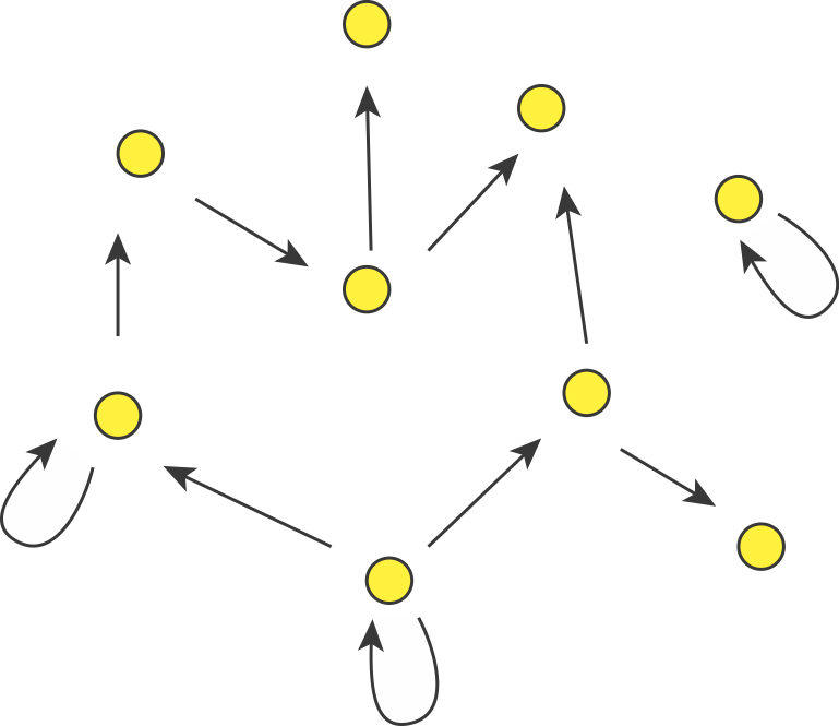
Consider a directed graph representing a hypothetical regulatory circuit (left). To find over-represented patterns in this graph, we can compare it to an ensemble of randomized variants and look for sub-graphs that occur more frequently in this circuit than in most of the variants.

Schematic comparison between a specific circuit (left) and a set of randomized variants with the same incoming and outgoing arrow distributions (right). Image modified fromMilo et al, Science, 2002.

To make the comparison as fair as possible, we need to design variant graphs that maintain the key statistical properties of the original graph. Specifically, we insist that all variant graphs have the same number of nodes and arrows. But this is not really enough: It wouldn’t make sense to compare this graph, whose arrows are distributed over all the nodes to a variant in which, say, all arrows stem from a single source node, or converge on a single target node. Therefore, we also need to impose a stronger constraint: maintaining the exact distribution of incoming and outgoing arrows for each node.

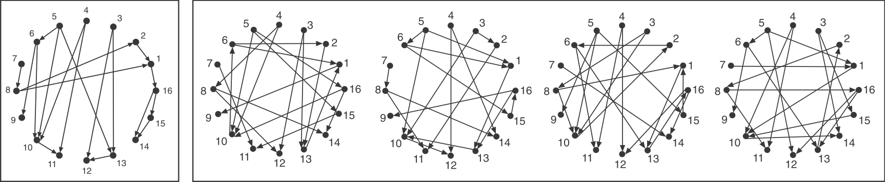
If you examine the graphs above, you can see that they were constructed to have the same numbered nodes. Furthermore, the number of arrows exiting and entering each numbered node is exactly the same in all graphs. For example, node 4 always has 2 outgoing arrows. Node 6 always has one incoming and two outgoing arrows, node 12 always has 2 incoming arrows, and so on.

To generate the randomized graphs, imagine cutting each arrow in half with a scissors to generate a dangling “+” end connected to an arrowhead and a dangling “-” end connected to a source node. Then one would tie each “+” end to a randomly chosen “-” end. Voila, a new randomized graph is guaranteed, through this procedure, to maintain the same joint distribution of incoming and outgoing arrows. For more details, see the algorithms in Shen-Orr et al, Nat. Genet., 2002 and in M. E. J. Newman et al, Phys. Rev. E, 2001.

To implement this type of algorithm, as described in Milo et al, Science, 2002, it is useful to represent the directed graph as a binary non-symmetric square matrix, \(\mathsf{M}\). An example of a matrix representation of a graph is shown below. Here, an arrow from node \(i\) to node \(j\) is represented by \(M_{i,j}=1\). The absence of such an arrow would be represented by \(M_{i,j}=0\). (This type of matrix, representing a corresponding graph, is called an adjacency matrix.) With this algorithm, one can generate a large ensemble of randomized graphs. Then, one can ask which sub-graphs are significantly more (or less) prevalent in the actual graph than in the randomized variant graphs.

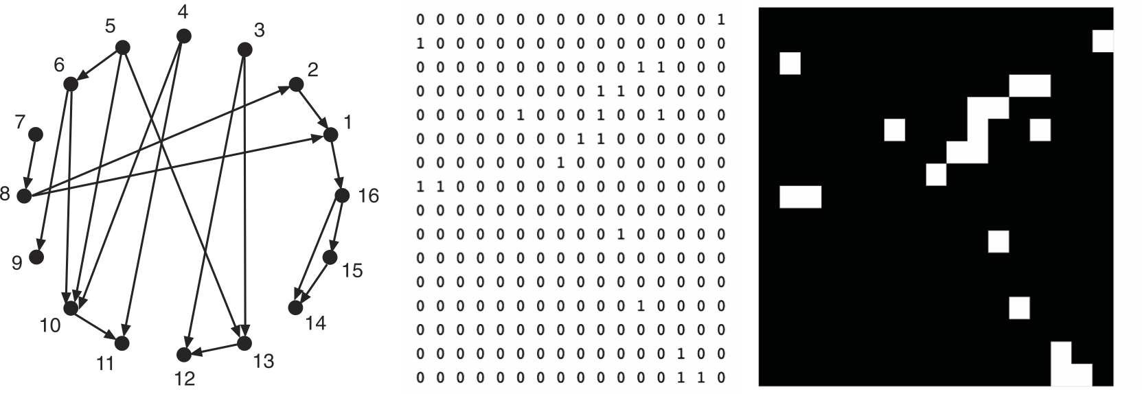
Different views of the same graph, using dots and arrows (left) or as a binary matrix, shown either with 0s and 1s or in black and white (right).

Questions: - What algorithm would you use to generate the randomized graphs (matrices)? - How would you control for the bias of smaller motifs in the frequency of larger motifs?

Finding 3-node motifs in a bacterial transcriptional network¶

Now that we have an algorithm to identify motifs, let’s use it on the E. coli network. First we will focus on 3-node sub-graphs. These are big enough to be quite interesting, but small enough to be easily conceptualized and analyzed. There are 13 possible 3-node graphs that exclude direct autoregulation, which are shown here in a drawing from the Alon book.

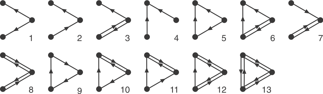
Image adapted fromMilo, et al., Science, 2002.

Now look back at the schematic graph/matrix representation above. Can you tell which of these sub-graphs are over-represented? That graph was constructed to contain a preponderance of one particular sub-graph:

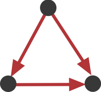
This sub-graph, termed the Feed-Forward Loop (FFL), has one node that regulates a target node two ways: directly, and indirectly through the third node.

To visualize this, we can highlight in red all of the FFLs in the graphs shown above, the one at left being artificially constructed and those to the right being randomly generated graphs.

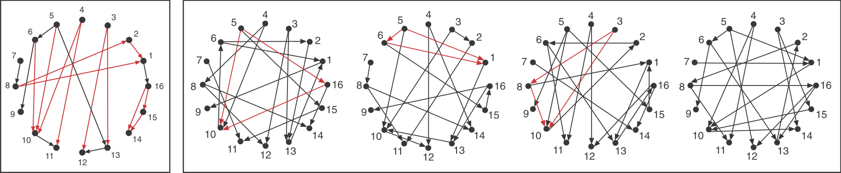
Image adapted fromMilo, et al., Science, 2002.

We see that the FFL motif is over-represented. Of course, this is a schematic graph deliberately constructed to illustrate over-representation of this sub-graph.

What happens in real circuits?

To address this question, Alon & colleagues went through the E. coli transcriptional circuit, and systematically counted how many times they observed each of the thirteen possible three-node sub-graphs shown above. For each one, they compared the number of observations in the real circuit to the number of times that sub-graph was observed in each member of a large ensemble of randomized circuits. They used a z-score to quantify over- or under-representation in units of the standard deviation of the number of occurrences for the sub-graph in the randomized circuits: \(z = (n_{obs}-\langle n\rangle)/\sigma\), where \(n_{obs}\) is the number of times the sub-graph was observed in the actual circuit, \(\langle n\rangle\) and \(\sigma\) denote the mean and standard deviation of the number of times it was observed in each of the randomized circuits.

They did this for several transcriptional circuits, including E. coli, yeast (two versions), and B. subtilis. Here are the results:

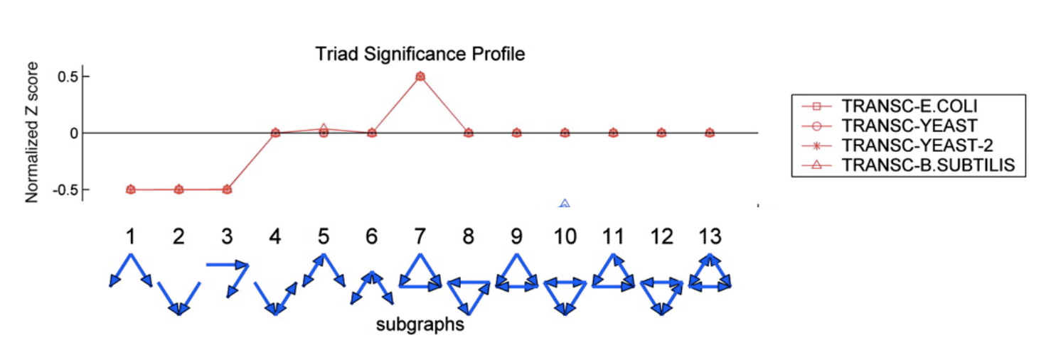
Image adapted fromMilo, et al., Science, 2004.

Several features are striking in this plot:

There is strong over-representation of feed-forward loops (FFLs). In E. coli, one expects to see 7±5 FFLs by chance, but one observes this pattern 42 times in the real circuit.
The over-representation of FFLs is conserved across three distinct organisms, suggesting it is a general property of transcriptional circuits.
Most other sub-graphs are neither over- nor under-represented.
Three sub-graphs are statistically under-represented. They occur significantly less often than one would expect by chance, provoking the question of what problems they might present as components of larger circuits. These three sub-graphs are all sub-graphs of the FFL sub-graph. Thus, it’s not that divergent regulation (sub-graph 1) is rare, it’s just that when it does occur, it does so in the context of the FFL.

How do sub-graph abundances scale?¶

Some species have much larger genomes than others. How would you expect the number of instances of different sub-graphs to change with the size of the overall circuit? You might at first think that larger circuits would simply have more copies of all possible sub-graphs. However, this is not the case. To see why, let’s try to get a better intuition for how often we expect to see various sub-graphs appear in graphs of different sizes.

We will ask: What is the probability of obtaining an n-vertex sub-graph, \(G\), by chance in a large random graph with \(N\) nodes and \(E\) edges? Clearly the answer will depend on the number of nodes, \(n\), and edges, \(g\), in \(G\). For the FFL, \(n=3, g=3\).

Many biological networks are sparse, meaning the probability, \(p\), of any potential edge occurring is low. Since the number of possible edges is \(N^2\), so that \(p = E/N^2 \ll 1\). For E. coli, \(p≈0.002\). We will therefore focus on this regime.

The question then becomes, for large sparse graphs, how should the expected number of occurrences of sub-graph, \(G\), scale with the size of the circuit, or number of nodes, \(N\)?. For this argument, we will ignore numerical prefactors, and focus only on the dependence on \(N\).

Within the overall network the number of potential instances of \(G\) is the binomial coefficient \(\binom{N}{n}\), where \(n\) is the number of nodes in \(G\), e.g. \(n=3\) for the FFL.
The probability that any one of these potential instances is the desired sub-graph, is proportional to \(p^g\), where \(g\) denotes the number of edges in the \(G\), e.g. \(g=3\) for the FFL. There is also a permutation factor, representing the number of different ways that you could make the desired sub-graph from a set of 3 nodes. We neglect this factor because it is independent of \(N\).
Since \(N \gg n\), we can use the well-known Stirling approximation of the binomial coefficient: \begin{align} \phantom{blah} \\ \binom{N}{n} \approx \frac{N^n e^n}{\sqrt{2\pi} n^{n+1/2}}\\[1em] \phantom{blah} \end{align} This is \(N^n\) times numerical factors that are independent of \(N\).
Thus, the expected number of occurrences scales as \(N^n p^g\).
Rewriting this expression provides more insight into the scaling of sub-graph abundance: \begin{align} &\phantom{blah} \\ N_G & \sim N^n p^g \\[1em] &= N^n \left( \frac{E}{N^2} \right)^g \\[1em] &= N^{n-2g} E^g \\[1em] &= N^{n-g} \left( \frac{E}{N} \right)^g\\[1em] \phantom{blah} \end{align} The thing to notice here is that the N-dependence can be captured by an extensive term that scales as \(N^{n-g}\) times a function fo the graph’s mean connectivity, \(E/N\), which is an intensive (N-independent) property.

This result leads to interesting and counterintuitive expectations:

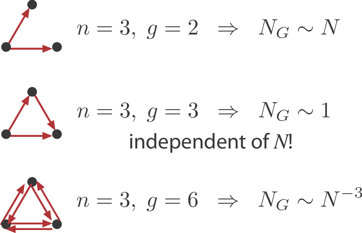
Sparsely connected sub-graphs increase in frequency with \(N\)
Densely connected sub-graphs decrease in frequency with \(N\). This means that as the graph grows larger there are actually fewer of these motifs.
And in between, sub-graphs with the same number of nodes and edges, such as the FFL, actually have a constant expected number regardless of \(N\).

Those last two points initially struck me as very counter-intuitive. How can the absolute number of times a graph appears in the network be independent of the size of that network? Surely, if you have more network you should have more of all subgraphs. But, loosely speaking, as the number of nodes increases the probability of an arrowhead landing on a node within a potential sub-graph decreaes.

Beyond transcriptional circuits¶

It’s important to remember that these are expectations for (a particular class of) random networks. Real networks will of course differ, because they are designed, or evolved, to perform specific functions. In fact, different types of systems seem to show quite distinct motif profiles:

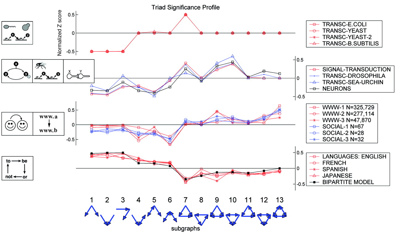
Image taken fromMilo, et al., Science, 2004

Here, the top group are the transcriptional circuits we already saw. The next group are biological signal transduction circuits of different types from different species. The third group are networks like the world-wide web, for which a directed edge indicates a link from one web page to another. Finally, the lowest group represents motifs in language graphs, in which nodes are words and edges are derived from the probability that one word follows another.

There are many kinds of FFLs¶

Our description of regulatory interactions so far has been oversimplified in several ways: * We have collapsed positive and negative regulation together. * We have not considered how multiple regulators combine to control expression of a mutual target operon. * We have ignored the quantitative strength of the regulation.

Understanding the function of a motif requires thinking about these aspects more carefully.

We can classify the overall FFL motif into \(2^3=8\) different categories depending on which of its 3 arrows are positive or negative:

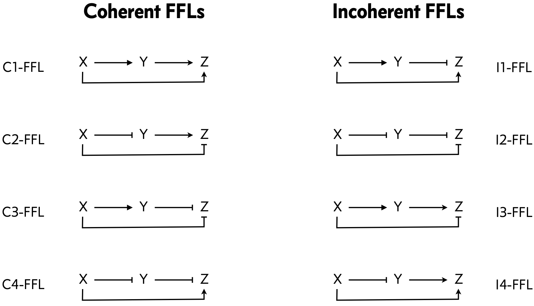
We can then further classify the FFLS, according to how the regulatory arrows converging on the third node (now labeled “Z”) combine. In AND regulation, both X and Y need to be simultaneously present at high levels for Z to be expressed. in OR regulation, either input is sufficient to activate Z.

In the next chapter, we will consider what functions the various FFLs can perform for cells.

Summary¶

Motifs are statistically over-represented patterns in a circuit.
To find motifs, we construct ensembles of random circuits with the same arrow distributions for comparison.
The abundances of different sub-graphs can scale in opposite and even counter-intuitive ways as the size of the overall circuit grows
This approach can be applied to a wide variety of systems that can be represented as graphs.
Transcriptional regulatory circuits appear to have a single major motif: the feed-forward loop.
There are multiple types of FFLs.

In the next chapter, we will explore the functions of this motif.